

-
摘要: 传统基于肌电(Electromyography,EMG)的运动识别方法多是利用训练后的固定参数模型,分类已预先定义的有限个目标动作,但对肌肉疲劳导致的肌电变化,以及未定义的外部动作等干扰因素无能为力.针对这一问题,提出一种自更新混合分类模型(Self-update hybrid classification model,SUHC),该模型融合了用于排除外部动作干扰的一类支持向量机(Support vector machine,SVM),以及用于分类目标动作数据的多类线性判别分析(Linear discriminant analysis,LDA),并引入自更新机制以对抗肌电时变性干扰.通过手部动作识别实验验证提出方法的效果,在肌电大幅变化干扰下,SUHC的目标动作识别精度达到89%,对比传统的支持向量机、多层感知器(Multiple layer perceptron,MLP)和核线性判别分析(Kernel LDA,KLDA),提高了约18%,并且SUHC具备排除外部动作干扰能力,排除精度高达93%.Abstract: The traditional electromyography (EMG)-based motion recognition methods always classify a limited number of pre-defined target motions by using a trained parameter-fixed model. However, those methods have no ability to handle the interference factors, including changes of EMG signals caused by muscle fatigue and outlier motions undefined beforehand. For this problem, a self-update hybrid classification model (SUHC) is proposed. In the SUHC, the one-class support vector machine (SVM) that can reject outlier motions is combined to a multi-class linear discriminant analysis (LDA) that is used to recognize target motions; furthermore, a self-update mechanism is adopted to reduce the influence caused by EMG changes. The performance of the proposed method is verified by the experiment of EMG-based hand motion recognition. Under the interference that EMG signals vary greatly, the recognition accuracy of SUHC on target motions is about 89%, which is 18% higher than those of the normal SVM, multiple layer perceptron (MLP) and kernel LDA (KLDA); moreover, the SUHC has the ability to reject outlier motions with a 93% of rejection accuracy.
-
-
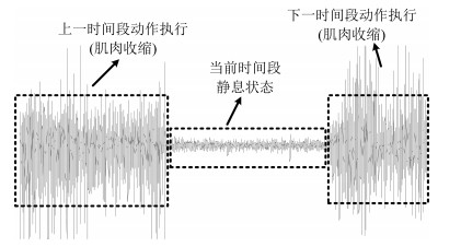
图 2 肌肉收缩及静息状态下, 采集的连续sEMG
Fig. 2 The continuous sEMG signals sampled at the states of muscle contraction and resting
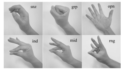
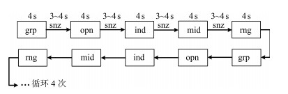
图 4 识别的5种手部动作以及手部休息姿势snz
Fig. 4 The five kinds of hand motions and the snooze state (snz) that were recognized in the paper

图 5 选取的肌肉及布置的采集电极,其中ch-$i$, $i = 1, 2, 3, 4$, 表示第$i$通道电极
Fig. 5 The selected muscles and the placement of electrodes, where ch-$i$ ($i = 1, 2, 3, 4$) represents the $i$th channel electrode
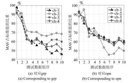
图 8 由10组测试样本数据计算的MAV占其标准值比
Fig. 8 The ratio of MAV with respect to the standard value calculated by using the ten sessions of test data

图 9 将Subject-1的第1组训练数据输入SUHC (仅给出该组数据的前2个循环), 实现模型在线更新
Fig. 9 Online updating the SUHC by inputting the first session of training data of Subject-1 into the model (only plot the first two cycles of the data)
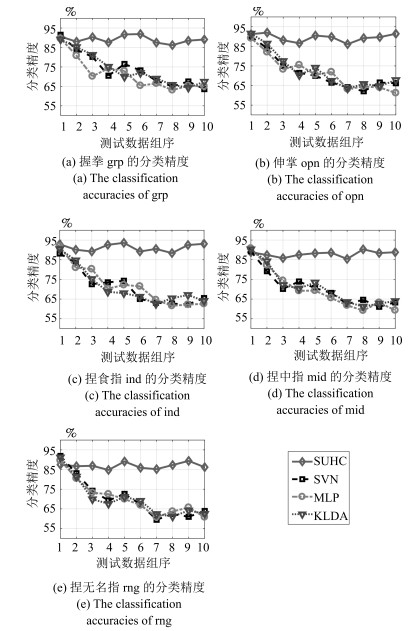
图 10 无外部动作干扰情况下, 使用Subject-1的10组测试数据计算的分类精度
Fig. 10 In the case of no outlier-motion interference, the classification accuracies calculated by using the ten sessions of test data of Subject-1

图 11 使用Subject-1的1组测试数据获得的动作识别结果
Fig. 11 The motion recognition results obtained by using one session of test data of Subject-1

图 12 存在外部动作(rng)干扰情况下, 使用Subject-1的10组测试数据获得的识别结果
Fig. 12 In the case of outlier-motion (rng) interference, the recognition results obtained by using ten sessions of test data of Subject-1

图 13 使用Subject-1的测试数据, 计算的分类精度与排除精度的均值和标准差
Fig. 13 The means and standard deviations of classification and rejection accuracies computed by using the test data of Subject-1
表 1 使用所有测试者的10组测试样本计算的平均分类精度与标准差(%)
Table 1 The mean classification accuracies and standard deviations calculated by using the ten sessions of test data of all subjects (%)
SUHC SVM MLP KLDA 1 ${\bf{91.5\pm4.3}}$ $89.3\pm5.1$ $90.4\pm2.9$ $89.8\pm5.9$ 2 ${\bf{89.1\pm2.6}}$ $85.1\pm7.5$ $81.7\pm6.4$ $83.4\pm8.1$ 3 ${\bf{88.7\pm6.6}}$ $75.3\pm10.4$ $74.3\pm8.8$ $77.1\pm10.7$ 4 ${\bf{86.2\pm4.1}}$ $70.8\pm14.4$ $71.2\pm10.7$ $72.7\pm11.2$ 5 ${\bf{93.4\pm3.8}}$ $73.0\pm9.1$ $70.7\pm13.5$ $71.5\pm14.6$ 6 ${\bf{88.5\pm6.2}}$ $69.8\pm12.9$ $64.2\pm11.2$ $67.3\pm11.9$ 7 ${\bf{86.0\pm5.7}}$ $59.9\pm12.3$ $59.5\pm12.1$ $62.1\pm13.4$ 8 ${\bf{88.1\pm8.4}}$ $61.7\pm10.2$ $57.8\pm13.0$ $59.4\pm14.7$ 9 ${\bf{91.4\pm4.9}}$ $58.4\pm9.7$ $60.1\pm10.6$ $61.6\pm9.2$ 10 ${\bf{87.9\pm4.3}}$ $62.8\pm10.3$ $57.0\pm15.6$ $58.1\pm13.9$ $m\pm st$ ${\bf{89.1\pm5.1}}$ $70.6\pm10.2$ $68.7\pm10.5$ $70.3\pm11.4$  下载: 导出CSV
表 2 使用所有测试者的测试数据计算的分类精度与排除精度的均值和标准差(%)
Table 2 The means and standard deviations of classification and rejection accuracies computed by using the test data of all subjects (%)
目标动作分类精度 外部动作排除精度 SUHC $90.4\pm4.4$ $93.5\pm3.0$ SVDD $82.1\pm8.7$ $91.9\pm5.2$ SVM $62.5\pm16.1$ $-$ MLP $60.8\pm18.4$ $-$ KLDA $60.1\pm15.7$ $-$
下载: 导出CSV
-
[1] 侯增广, 赵新刚, 程龙, 王启宁, 王卫群.康复机器人与智能辅助系统的研究进展.自动化学报, 2016, 42(12):1765-1779 http://www.aas.net.cn/CN/abstract/abstract18966.shtmlHou Zeng-Guang, Zhao Xin-Gang, Cheng Long, Wang Qi-Ning, Wang Wei-Qun. Recent advances in rehabilitation robots and intelligent assistance systems. Acta Automatica Sinica, 2016, 42(12):1765-1779 http://www.aas.net.cn/CN/abstract/abstract18966.shtml [2] Ding Q C, Han J D, Zhao X G. Continuous estimation of human multi-joint angles from sEMG using a state-space model. IEEE Transactions on Neural Systems and Rehabilitation Engineering, 2017, 25(9):1518-1528 doi: 10.1109/TNSRE.2016.2639527 [3] 胡进, 侯增广, 陈翼雄, 张峰, 王卫群.下肢康复机器人及其交互控制方法.自动化学报, 2014, 40(11):2377-2390 http://www.aas.net.cn/CN/abstract/abstract18514.shtmlHu Jin, Hou Zeng-Guang, Chen Yi-Xiong, Zhang Feng, Wang Wei-Qun. Lower limb rehabilitation robots and interactive control methods. Acta Automatica Sinica, 2014, 40(11):2377-2390 http://www.aas.net.cn/CN/abstract/abstract18514.shtml [4] 丁其川, 熊安斌, 赵新刚, 韩建达.基于表面肌电的运动意图识别方法研究及应用综述.自动化学报, 2016, 42(1):13-25 http://www.aas.net.cn/CN/abstract/abstract18792.shtmlDing Qi-Chuan, Xiong An-Bin, Zhao Xin-Gang, Han Jian-Da. A review on researches and applications of sEMG-based motion intent recognition methods. Acta Automatica Sinica, 2016, 42(1):13-25 http://www.aas.net.cn/CN/abstract/abstract18792.shtml [5] Tkach D, Huang H, Kuiken T A. Study of stability of time-domain features for electromyographic pattern recognition. Journal of Neuroengineering and Rehabilitation, 2010, 7:Article No. 21 doi: 10.1186/1743-0003-7-21 [6] 丁其川, 赵新刚, 韩建达.基于肌电信号容错分类的手部动作识别.机器人, 2015, 37(1):9-16 http://d.old.wanfangdata.com.cn/Periodical/jqr201501002Ding Qi-Chuan, Zhao Xin-Gang, Han Jian-Da. Recognizing hand motions based on fault-tolerant classification with EMG signals. Robot, 2015, 37(1):9-16 http://d.old.wanfangdata.com.cn/Periodical/jqr201501002 [7] Huang Y, Englehart K B, Hudgins B, Chan A D C. A Gaussian mixture model based classification scheme for myoelectric control of powered upper limb prostheses. IEEE Transactions on Biomedical Engineering, 2005, 52(11):1801-1811 doi: 10.1109/TBME.2005.856295 [8] Li G L, Schultz A E, Kuiken T A. Quantifying pattern recognition-based myoelectric control of multifunctional transradial prostheses. IEEE Transactions on Neural Systems and Rehabilitation Engineering, 2010, 18(2):185-192 doi: 10.1109/TNSRE.2009.2039619 [9] Liu J, Zhou P. A novel myoelectric pattern recognition strategy for hand function restoration after incomplete cervical spinal cord injury. IEEE Transactions on Neural Systems and Rehabilitation Engineering, 2013, 21(1):96-103 doi: 10.1109/TNSRE.2012.2218832 [10] 郭欣, 王蕾, 宣伯凯, 李彩萍.基于有监督Kohonen神经网络的步态识别.自动化学报, 2017, 43(3):430-438 http://www.aas.net.cn/CN/abstract/abstract19021.shtmlGuo Xin, Wang Lei, Xuan Bo-Kai, Li Cai-Ping. Gait recognition based on supervised Kohonen neural network. Acta Automatica Sinica, 2017, 43(3):430-438 http://www.aas.net.cn/CN/abstract/abstract19021.shtml [11] Artemiadis P K, Kyriakopoulos K J. An EMG-based robot control scheme robust to time-varying EMG signal features. IEEE Transactions on Information Technology in Biomedicine, 2010, 14(3):582-588 doi: 10.1109/TITB.2010.2040832 [12] Duan F, Dai L L. Recognizing the gradual changes in sEMG characteristics based on incremental learning of wavelet neural network ensemble. IEEE Transactions on Industrial Electronics, 2017, 64(5):4276-4286 doi: 10.1109/TIE.2016.2593693 [13] Kato R, Yokoi H, Arai T. Real-time learning method for adaptable motion-discrimination using surface EMG signal. In: Proceedings of the 2006 IEEE/RSJ International Conference on Intelligent Robots and Systems. Beijing, China: IEEE, 2006.2127-2132 [14] Yang D P, Jiang L, Liu R Q, Liu H. Adaptive learning of multi-finger motion recognition based on support vector machine. In: Proceedings of the 2013 IEEE International Conference on Robotics and Biomimetics (ROBIO). Shenzhen, China: IEEE, 2013.2231-2238 http://ieeexplore.ieee.org/xpls/abs_all.jsp?arnumber=6739801 [15] Chen X P, Zhang D G, Zhu X Y. Application of a self-enhancing classification method to electromyography pattern recognition for multifunctional prosthesis control. Journal of NeuroEngineering and Rehabilitation, 2013, 10:Article No. 44 doi: 10.1186/1743-0003-10-44 [16] Anam K, Al-Jumaily A. A robust myoelectric pattern recognition using online sequential extreme learning machine for finger movement classification. In: Proceedings of the 37th Annual International Conference of the IEEE on Engineering in Medicine and Biology Society (EMBC). Milan, Italy: IEEE, 2015.7266-7269 http://www.ncbi.nlm.nih.gov/pubmed/26737969 [17] Scheme E J, Englehart K B, Hudgins B S. Selective classification for improved robustness of myoelectric control under nonideal conditions. IEEE Transactions on Biomedical Engineering, 2011, 58(6):1698-1705 doi: 10.1109/TBME.2011.2113182 [18] Li Z J, Wang B C, Yang C G, Xie Q, Su C Y. Boosting-based EMG patterns classification scheme for robustness enhancement. IEEE Journal of Biomedical and Health Informatics, 2013, 17(3):545-552 doi: 10.1109/JBHI.2013.2256920 [19] Liu Y H, Huang H P. Towards a high-stability EMG recognition system for prosthesis control: a one-class classification based non-target EMG pattern filtering scheme. In: Proceedings of the 2009 IEEE International Conference on Systems, Man, and Cybernetics. San Antonio, USA: IEEE, 2009.4752-4757 [20] Ding Q C, Li Z Y, Zhao X G, Xiao Y F, Han J D. Real-time myoelectric prosthetic-hand control to reject outlier motion interference using one-class classifier. In: Proceedings of the 32nd Youth Academic Annual Conference of Chinese Association of Automation (YAC). Hefei, China: IEEE, 2017.96 -101 http://ieeexplore.ieee.org/document/7967385/ [21] Tax D M J, Duin R P W. Support vector data description. Machine Learning, 2004, 54(1):45-66 http://d.old.wanfangdata.com.cn/Periodical/xajtdxxb200309008 [22] Tax D M J, Laskov P. Online SVM learning: from classification to data description and back. In: Proceedings of the 13th IEEE Workshop on Neural Networks for Signal Processing. Toulouse, France: IEEE, 2003.499-508 http://ieeexplore.ieee.org/xpls/icp.jsp?arnumber=1318049 [23] Cauwenberghs G, Poggio T. Incremental and decremental support vector machine learning. In: Proceedings of the 2000 International Conference on Neural Information. Cambridge, USA: MIT Press, 2000.388-394 http://dl.acm.org/citation.cfm?id=3008808 [24] Bishop C. Pattern Recognition and Machine Learning. New York, USA:Springer, 2006. [25] Futamata M, Nagata K, Magatani K. The evaluation of the discriminant ability of multiclass SVM in a study of hand motion recognition by using sEMG. In: Proceedings of the 2012 Annual International Conference on Engineering in Medicine and Biology Society (EMBC). San Diego, USA: IEEE, 2012.5246-5249 [26] Amsuss S, Goebel P M, Jiang N, Graimann B, Paredes L, Farina D. Self-correcting pattern recognition system of surface EMG signals for upper limb prosthesis control. IEEE Transactions on Biomedical Engineering, 2014, 61(4):1167 -1176 doi: 10.1109/TBME.2013.2296274 [27] Mika S, Rätsch G, Weston J, Schölkopf B, Muller K R. Fisher discriminant analysis with kernels. In: Proceedings of the 1999 IEEE Signal Processing Society Workshop, Neural Networks for Signal Processing. New York, USA: IEEE, 1999.41-48 http://ieeexplore.ieee.org/xpls/abs_all.jsp?arnumber=788121 [28] Baudat G, Anouar F. Generalized discriminant analysis using a kernel approach. Neural Computation, 2000, 12(10):2385-2404 doi: 10.1162/089976600300014980 [29] Shahbaba B. Biostatistics with R:An Introduction to Statistics through Biological Data. New York:Springer, 2012.221 -234 [30] Ding Q C, Han J D, Zhao X G, Chen Y. Missing-data classification with the extended full-dimensional Gaussian mixture model:applications to EMG-based motion recognition. IEEE Transactions on Industrial Electronics, 2015, 62(8):4994-5005 doi: 10.1109/TIE.2015.2403797 -


计量
- 文章访问数: 1583
- HTML全文浏览量: 239
- PDF下载量: 125
- 被引次数: 0
