

Target Segmentation of Infrared Image Using Fused Saliency Map and Efficient Subwindow Search
-
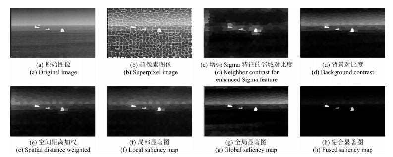
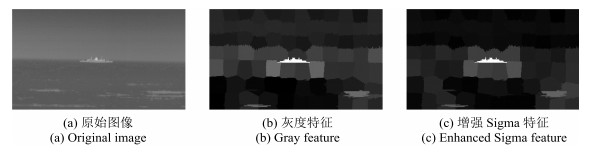
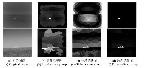
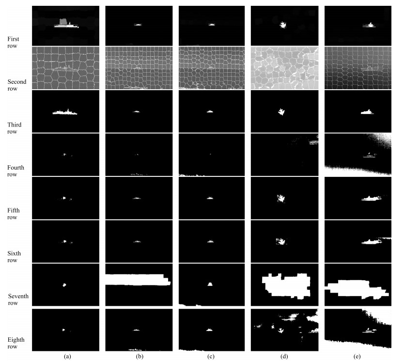
摘要: 为了快速精确地分割红外图像目标,提出一种基于融合显著图和高效子窗口搜索的红外目标分割方法.在获取图像超像素的基础上,提取每个区域增强的Sigma特征,并考虑邻域对比度、背景对比度、空间距离和区域大小的影响,构建局部显著图,接着利用全局核密度估计构建全局显著图,然后融合局部和全局显著图实现图像显著性检测,最后应用高效子窗口搜索方法检测和筛选目标,实现红外目标分割.实验结果表明,新方法的显著图结果目标区域一致高亮且边缘清晰,背景杂波抑制效果好,可实现快速精确的目标分割.Abstract: In order to segment infrared target fast and precisely, a segmentation method using fused saliency map and efficient subwindow search is proposed. Firstly, based on image superpixels, the enhanced sigma feature of every region is extracted, and at the same time considering the influence of neighbor contrast, background contrast, spatial distance and region's size, the local saliency map is constructed. Next, the global saliency map is obtained by global kernel density estimation. Then, the saliency detection result of infrared image is obtained by fusing the local and global saliency maps. Finally, the efficient subwindow search method is used to detect and segment the target. Experimental results show that the saliency map of the proposed method has complete target feature, obvious edges and good background suppression, and that the algorithm can segment the infrared target fast and precisely.
-
混合动力电动汽车(Hybrid electric vehicle, HEV)是配备了两种或两种以上动力源(其中一种动力由电动机提供)的汽车, 它具备传统汽车和纯电动汽车两者的优点.通过不同能源的优化互补、协调合作, 可在保证汽车动力性、安全性及舒适性的前提下, 改善汽车的节能减排性能.由于电池技术尚未取得突破性进展, 因此混合动力电动汽车成为汽车厂商和研究机构关注与研究的热点.
混合动力电动汽车通常采用两种动力源, 动力源之一是传统发动机(柴油机、汽油机或燃汽轮机), 另一种动力源由电机电池组、燃料电池、飞轮等提供.本文主要研究电机电池与发动机组合的混合动力汽车.与纯电动汽车相比, 混合动力电动汽车具有多方面的优越性.混合动力电动汽车充分利用了发动机与电动机的工作特性, 通过协调发动机与电池/电机组的能源分配, 保证发动机工作在高效低能耗区, 还可利用电动机的再生制动, 回收尽可能多的能量.因此, 混合动力电动汽车缓解了纯电动汽车电池储能有限、续航能力低的技术瓶颈.另外, 混合动力电动汽车可避免在城区工况下频繁起停, 减少车辆怠速行驶工况, 可实现比传统内燃机汽车更优异的燃油经济性和清洁环保性.同时, 混合动力汽车结构多样, 可通过对传统汽车结构的较小改动而实现混合动力车的设计, 大大降低了设计的复杂程度.与传统汽车相比, 混合动力电动汽车可在保证行驶性能和不损失使用寿命的前提下, 通过合理的结构配置, 降低发动机等构件的重量及成本.
混合动力电动汽车包含了电能、热能、机械能之间的能量转换与控制关系, 其分类有多种方式.根据混合动力电动汽车的混合程度可分为微混式混合动力、轻混式混合动力和全混式混合动力[1].根据混合动力电动汽车的结构可分为串联式混合动力、并联式混合动力与混联式混合动力[2], 而对于并联或混联式混合动力电动汽车, 根据动力源输出动力耦合方式的不同可分为转速耦合式混合动力、扭矩耦合式混合动力、功率耦合或混合耦合[3-4], 转速耦合其特点是动力装置的转速是解耦的, 发动机的转矩不可控, 而发动机的转速则可通过电机的转速进行控制; 转矩耦合方式的特点是发动机的转矩可控, 而发动机转速不可控, 往往通过电机转矩控制实现发动机转矩控制, 使发动机工作在最佳油耗曲线附近; 功率耦合也被称之为混合耦合, 指包含两种或以上扭矩耦合与转速耦合的耦合方式, 其发动机的转矩和转速均不受汽车工况的影响, 都是可控的.无论哪种类型的混合动力电动汽车都是非常复杂的非线性系统, 对控制策略都提出了极高的要求.能量管理系统作为混合动力电动汽车的核心, 其能量管理策略的优劣直接影响着混合动力电动汽车的可靠性、控制性、经济性和排放性能.因此, 能量管理始终是混合动力电动汽车领域的重点研究课题, 其控制方法层出不穷.早期的能量管理方法采用基于规则的控制方法[2, 5-7], 后来广泛采用了基于动态规划的能量管理算法[8-12].近年来, 各种先进智能化能量管理方法不断涌现, 代表性的方法包括实时等效油耗控制算法[13-19]、预测模型控制算法[20-25]、最优控制算法[26-28]以及模糊控制算法[5, 29-41]、神经网络控制算法[32-33, 42-43]、遗传算法[15, 44-46]等智能控制方法.
本文首先总结了研究人员从不同角度对混合动力电动汽车的能量管理问题所做的定义和描述, 然后对不同问题体系下的各种已有能量管理策略加以梳理分类研究, 深入分析了各种控制方法的特点及其存在的问题和不足, 并对未来推进混合动力电动汽车能量管理研究的发展方向和初步思路做了展望.
1. 能量管理问题的描述
能量管理策略是混合动力电动汽车的核心技术, 是实现车辆燃油经济性和清洁环保性的关键.只有在充分了解不同动力源工作原理及工作特性的基础上, 合理利用两种动力源的优势, 采取行之有效的控制策略才能达到预想的控制目标.混合动力电动汽车能量管理策略对于能量的节省与效率的优化主要体现在以下几个方面:
1) 考虑电机电池组响应快、低速输出扭矩大; 而发动机响应慢、起动扭矩小等特点, 利用电机实现车辆的快速起步或加速, 保证发动机始终工作于高效率区, 弥补车辆功率峰值的波动需求, 实现发动机的高效率低排放;
2) 实现部分工况下的纯电动行驶, 使发动机在相应工况下实现零能耗零排放;
3) 汽车在下坡减速制动过程中利用电动机回收制动过程中的能量损耗对电池进行充电;
4) 利用电机的快速起停特性, 避免发动机经常处在城市怠速工况下而产生高油耗与高排放.
由于混合动力电动汽车能量管理涉及了电能、热能、机械能等能量的转化与控制, 系统十分复杂, 并且其控制优化目标也各有不同.因此, 大量的文献从不同的角度对混合动力电动汽车能量管理问题进行了定义与描述.一类是基于规则的能量管理问题, 通常将问题描述为依据工程经验或实验数据确定发动机的工作区域, 通过电动机协调控制其工作模式, 制定规则以保证发动机在高效范围内工作.另一类是将其描述为不同优化目标的能量管理问题.大量的文献通过对两种动力的合理分配实现混合动力电动汽车的能量优化[15, 27-28, 47-49], 也有部分文献将电池荷电状态(State of charge, SOC)作为优化函数的约束条件[17, 21, 39]或其中的加权项[50-51], 还有的文献综合考虑了车辆的起动[21, 30]、换档[9, 30, 39]等瞬态过程的能量消耗以及车辆的驾驶性能[23, 52]、质量[26]、排放[8, 53-55]等因素, 将混合动力电动汽车能量管理问题描述为一个多目标综合优化问题.
一般地, 混合动力电动汽车的动态模型可表示为:
连续时间:
$ \dot{x}(t)=f(x(t), u(t)), \quad 0\leq t\leq T $
离散时间:
$ {x(k+1)}=f(x(k), u(k)), \quad k=1, 2, \cdots, N $
其能量管理问题可概括为如下优化问题:
$ \begin{align} &\min_{x, u}J(x, u)\\ &{\rm s.\, t.}\quad G(x)\leq0 \end{align} $
其中, $x\in X$ 为系统的状态变量, 通常表示为电池的电量SOC, $u\in U$ 表示控制变量, 通常为功率需求或转矩需求的分配比, $G(x)$ 表示约束条件, 比如, 电机的功率与转速限制、发动机转矩与转速限制、SOC终值约束等.
能量管理问题的控制目标由成本函数 $J(x, u)$ 表示, 考虑不同影响因素或不同优化目标的成本函数具有不同的选取和表达方式, 下面概括介绍文献中常见的几种成本函数的能量管理优化问题的表述形式.
1.1 等效油耗的能量管理问题
文献[13]将能量管理问题表达为发动机的油耗与电机等效油耗成本之和, 即把等效油耗控制问题表述为如下优化问题:
$ \begin{align} \min_{u}J(t, u)=\Delta E_f(t, u)+s(t)\Delta E_e(t, u) \end{align} $
其中, $\Delta E_f(t, u)$ 为 $\Delta t$ 时间内的发动机油耗, $\Delta E_e(t, u)$ 为 $\Delta t$ 时间内的电能消耗, 分别由发动机与电机Map图获得, $u$ 为控制转矩, $s(t)$ 为随时间变化的能量转化等效因子.
文献[14]为自适应等效油耗能量管理问题, 考虑在充、放电过程中其等效因子是不同的情况, 连续时间系统问题描述为
$ \begin{align} &\quad \min_{\{P_{ice}(t), P_{em}(t)\}}J=\dot m_{ice}(P_{ice}(t))+\zeta (P_{em}(t))\\ &{\rm s.\, t.}\quad {\rm If}\ P_{req}(t)\geq0, \\ &\qquad \ {P^{opt}_{ice}(t)=0, P^{opt}_{em}(t)=P_{req}(t)}\\ &\quad {\rm If}\, P_{req}(t) < 0, \\ &\quad \left\{\begin{array}{*{20}lll} P_{req}(t) = P_{ice}(t)+P_{em}(t)\\ {\rm SOC}_{\rm min} < {\rm SOC}(t) < {\rm SOC}_{\rm max}, \ \forall t\\ 0 \leq P_{ice}(t)\leq P_{ice, {\rm max}}(t)\\ P_{em, {\rm min}}(t)\leq P_{em}(t)\leq P_{em, {\rm max}}(t)\end{array}\right. \end{align} $
其中, $P_{req}(t)$ 为功率需求, $P_{ice}(t)$ 为发动机功率, $P_{em}(t)$ 表示电机功率, $\dot m_{ice}(P_{ice}(t))$ 为发动机的燃油消耗, $\zeta (P_{em}(t))$ 表示电能转化的等效油耗, SOC $(t)$ 为电池荷电状态.
1.2 考虑SOC的能量管理问题
考虑到电池容量和健康问题, 许多混合动力电动汽车能量管理问题都考虑了电池的SOC.文献[39, 54-56]引入了SOC约束条件, 即要求SOC工况循环终了值等于初始值; 文献[14, 18, 21, 42]将SOC约束在一定的范围内; 文献[8, 22, 30, 40, 57]将其转化为成本函数的加权项.文献[17]除了考虑了SOC约束, 同时还考虑了SOH(State of health)问题, 其能量管理优化问题表述为
$ \begin{align} & \min_{u}: \int_{0}^{T}P_f(u, v, a, t){\rm d}t \\ {\rm s.\, t.} \quad & \dot x_1(t)=\frac{-P_i(u(t))}{Q_0(t)}\\ &\dot x_2(t)=\frac{-\vert P_i(u(t))\vert}{(2\cdot N(\vert P_i(u(t))\vert)\cdot Q_0(0))}\\ & x_1(0)=x_{1, 0}\\ & x_2(0)=1\\ & x_1(T)\geq x_{1, 0}\\ & x_2(T)\geq0\\ & x(t)\in X, x=[x_1, x_2]^{\rm T}\\ & u(t)\in U \end{align} $
其中, $P_f(u, v, a, t){\rm d}t$ 表示能量消耗率, $x_1(0)$ 、 $x_2(0)$ 与 $x_1(T)$ 、 $x_2(T)$ 分别表示SOC与SOH的初始与终了值, $P_i(u(t))$ 表示电池输出功率, $x_{1, 0}$ 与 $Q_0(0)$ 表示电池初始的SOC与容量, $X$ 、 $U$ 为状态量和控制量空间.
1.3 考虑排放的能量管理问题
随着环境污染的加剧, 车辆排放问题成了继能源问题之后的又一关注热点.因此, 将排放纳入到成本函数形成燃油消耗与排放控制的折衷优化问题.文献[8, 46]将能源管理问题表示为燃油消耗和排放指标构成的综合性能指标, 并考虑SOC状态, 形成如下多目标优化问题:
$ \begin{align} &J=\sum_{k=0}^{N-1}[L(x(k), u(k))+G(x(N))]\\ &L(x(k), u(k))=fuel(k)+\mu NOx(k)+vPM(k)\\ &G(x(N))=\alpha({\rm SOC}(N)-{\rm SOC}_f)^2 \end{align} $
其中, $fuel(k)$ 为第 $k$ 时间段的燃油消耗, $NOx(k)$ 、 $PM(k)$ 为 $NOx$ 、 $PM$ 的排放量, ${\rm SOC}_f$ 为期望的荷电状态SOC的终值, $\mu$ 、 $v$ 、 $\alpha$ 为加权因子, $L(x(k), u(k))$ 表示为燃油消耗与排放, $G(x(N))$ 表示SOC的变化影响.
1.4 考虑瞬时工况油耗的能量管理问题
车辆在城市工况下行驶, 经常处于起停、换挡等瞬态工况, 为了提高燃油经济性, 有必要考虑过渡工况对燃油消耗的影响.文献[9]考虑了挡位切换对能耗的影响, 将优化问题表述为以价格表示的两种能源消耗:
$ \begin{align} &\min_{\{i_{k}\}k=0, 1, 2, \cdots, N-1}G=\sum_{k=0}^{N-1}\Delta Q_k+J_k\\ &\Delta Q_k=I_k U_k P_{r1}/1\, 000/3\, 600+b_{e, k} P_k P_{r2}/3\, 600/\rho\\ &J_k=\lambda\vert i_{k+1}-i_k\vert \end{align} $
其中, $k$ 为时间步, $i_k$ 表示挡位, $P_{r1}$ 表示电价格(元/kW $\cdot$ h), $P_{r2}$ 表示燃油价格(元/L), $\rho$ 为燃油密度, $P_k$ 表示电池功率, $U_k$ 、 $I_k$ 分别表示电池的端电压与电流, $b_{e, k}$ 为燃油消耗率, $\Delta Q_k$ 为以价格表示的两种能耗成本, $J_k$ 为传动比变化的影响.
文献[21]考虑了车辆起动瞬时工况, 将成本函数定义为发动机油耗、电池SOC变化的等效油耗与发动机起停时的瞬时油耗之和:
$ \begin{align} J(k)=~&\alpha_1\int_{t_k}^{t_k+t_p}\dot m_f(t){\rm d}t+\alpha_2[{\rm SOC}(t_k)-\\ &{\rm SOC}(t_k+t_p)]+\alpha_3[1-key\_on(t_k+t_p)]\\ {\rm s.\, t.} \quad &{\rm SOC}_{low\_lim} < {\rm SOC} < {\rm SOC}_{up\_lim} \end{align} $
其中, $\dot m_f(t)$ 表示发动机的燃油消耗率, $key\_on\in \{0, 1\}$ 代表发动机的状态, $\alpha_i, i=1, 2, 3$ 为加权系数, $t_k$ 为第 $k$ 步时刻, $t_p$ 为预测时间段, ${\rm SOC}_{up\_lim}$ 与 ${\rm SOC}_{low\_lim}$ 表示电池荷电状态SOC的上下界.
文献[30]不仅考虑了发动机稳态油耗、发动机起停时油耗, 还考虑了换挡时的油耗, 其成本函数选为发动机稳态油耗、发动机起停时油耗、换挡油耗、SOC保持的油耗的总和, 即:
$ \begin{align} J=\sum_{k=0}^{N-1}L(x(k), u(k))+L_e(k)+L_b(k)+G(x(N)) \end{align} $
其中
$ \begin{align} &L(x(k), u(k))=P_e(k)\cdot g_e(k)\cdot t\\ &L_e(k)=\alpha({\rm sgn}(n_e(k+1))- {\rm sgn}( n_e(k)))\\ &L_b(k)=\beta\vert i(k+1)-i(k)\vert\\ &G=\gamma({\rm SOC}(N)-{\rm SOC}(0))^2 \end{align} $
$L(x(k), u(k))$ 为发动机稳态油耗, $L_e(k)$ 为发动机频繁起停时引起的油耗, $L_b(k)$ 为发动机换挡时油耗, $G(x(N))$ 为SOC维持的能耗, $P_e(k)$ 表示发动机的功率, $g_e(k)$ 表示燃油消耗率, $t$ 表示间隔时长, $ signn_e(k)$ 表示发动机的状态, $i(k)$ 表示 $k$ 时刻的挡位, SOC $(0)$ 与SOC $(N)$ 分别表示电池荷电量的初始值与终了值, $\alpha$ 、 $\beta$ 、 $\gamma$ 为加权系数.
1.5 考虑结构参数影响的能量管理问题
车辆的质量、结构对系统的能耗都会产生重要的影响.文献[26]通过分析不同的结构, 构造了混合动力电动汽车油耗与质量间的折衷权衡问题, 其成本函数为两者的加权和, 即
$ \begin{align} J=\min(F\cdot w_f+W\cdot w_s) \end{align} $
其中, $F$ 为油耗, $W$ 为重量, $w_f$ 、 $w_s$ 为各自的加权值.
文献[39]考虑了不同的挡位对能耗的影响, 保证整个工况循环下的油耗最少, 形成如下全局最优问题:
$ \begin{align} & \min_{T_e(k), i(k)}J'=\sum_{k=0}^{N-1}D(T_e(k), i(k))\cdot\Delta\\ & D(T_e(k), i(k))=\dot m(T_e(k), w_e(k), R(i(k)))\\ {\rm s.\, t.}\quad &T'_{e\_min}(k)\leq T_e(k)\leq T'_{e\_max}(k), i(k)\in I(k)\\ & x(N)-x(0)=\Delta {\rm SOC}=0 \end{align} $
其中, $\Delta $ 为采样时间, $D(T_e(k), i(k))$ 为当发动机产生转矩为 $T_e(k)$ 、传动比为 $R(i(k))$ 时的油耗, $\dot m(T_e(k))$ 为当发动机转矩为 $T_e(k)$ 、转速为 $w_e(k)$ 时的油耗, 由发动机Map图计算获得, $i(k)$ 为挡位, $T'_{e\_max}(k)$ 与\ $T'_{e\_min}(k)$ 分别为发动机输出转矩的上下界, $x$ 为电池电量.
文献[23]以优化车辆工作效率达到提高串联混合动力燃油经济性的目的, 定义了如下优化问题:
$ \begin{align} &\eta_{sys}^*(P_{gen})=\max_{\omega_{eng}, \tau_{eng}}\eta_{sys}(\omega_{eng}, \tau_{eng})\\ & {\rm s.\, t.}\quad \eta_{gen}\left(\frac{\omega_{eng}}{k}, k\tau_{eng}\right)\omega_{eng}\tau_{eng}=P_{gen} \end{align} $
其中, $\eta_{sys}^*(P_{gen})$ 表示系统的优化目标, 即系统效率的最大值, $\eta_{sys}$ 为系统效率, $\eta_{gen}$ 表示电机效率, $\omega_{eng}$ 为发动机的转速, $\tau_{eng}$ 表示发动机的转矩, $P_{gen}$ 为电机功率, $k$ 为发动机与电机之间的传动比.
2. 混合动力电动汽车的能量管理策略研究进展
混合动力电动汽车能量管理问题根据控制目标与考虑因素的不同, 有多种描述形式.控制策略从不同的角度, 也有多种划分方式:根据结构形式[2]分为串联式混合动力电动汽车控制策略、并联式混合动力电动汽车控制策略; 从控制策略的实现角度分为直接法与间接法[1, 58]; 针对混合动力电动汽车能量优化的工作状态分为稳态优化控制策略与动态/实时优化控制策略[58]; 从控制策略的控制方式可概括为基于规则的控制方法和基于优化的控制方法[46].一些文献从不同的角度对混合动力电动汽车能量管理策略进行概括整理[1-2, 11, 53, 59-61].文献[58]主要针对混联式混合动力车辆的不同复合方式和结构方案进行介绍, 并从发动机恒定工作点模式、发动机最优工作曲线模式、瞬时优化模式、全局优化模式对控制算法进行了分类介绍.文献[2]介绍混合动力电动汽车的发展、分类、对比与发展趋势, 重点讨论了自2007年来的控制策略的分类及各自的优缺点.文献[1]主要是根据混合动力电动汽车的混合程度, 对微混式混合动力、轻微式混合动力、全混式混合动力电动汽车的控制技术进行了概述.文献[53]讨论了混合动力车辆能量管理系统优化所涉及的主要问题, 主要从结构的角度进行具体分析.文献[60]对1990年~2004年混合动力车辆的相关文献进行研究, 综述了HEV的能量优化控制策略, 概括了混合动力能量优化问题的数学描述(包括控制目标、控制器、约束条件、性能指标); 能量管理策略主要从静态优化、数字优化、分析优化、实时优化等方法进行概括.文献[11]综述了1998年~2014年HEV与Plug-in HEV的控制算法.首先给出了能量管理问题的数学描述, 然后以时间顺序分别对于串联式、并联式、混联式以及Plug-in混合动力车辆的控制策略按照在线与离线的控制方法进行介绍, 分析其优缺点并讨论未来研究方向与挑战.文献[61]综述了2012年之前的HEV/Plug-in HEV的控制策略.对其进行分类概括, 讨论了各种控制策略的优缺点.无论混合动力电动汽车采用哪种结构形式, 无论是基于稳态特性还是动态特性, 无论采用直接法还是间接法, 其控制方法都是多种多样的, 各有各自的特点, 存在着独特优势的同时也存在着一定的局限性, 因此也推动着混合动力电动汽车控制技术的发展, 不断地发现和解决问题的同时, 控制策略也不断地推陈出新.本文从控制方式的角度进一步对目前的混合动力电动汽车能量管理策略进行概括梳理, 总结分析各种控制策略的特点, 整理其发展脉络.图 1为混合动力电动汽车能量管理策略划分.
2.1 基于规则的能量管理策略
由于基于规则的能量管理策略, 其控制简单, 易于实现, 因而成为被最早用于混合动力电动汽车的控制方法.主要包含两种形式:一种是基于确定规则的控制方法, 根据不同的转矩、车速与SOC条件(如加速踏板、制动踏板指令)或其效率Map图, 对电机或发动机工作状态进行模式划分, 制定规则进行切换控制; 另一种是基于模糊逻辑的控制策略, 针对混合动力电动汽车具有多变量、非线性和时变的特点, 结合模糊控制的优势, 建立状态变量与状态变量变化率的隶属度函数, 确定模糊控制规则进行能量分配与SOC的控制.
2.1.1 基于确定规则的能量管理策略
基于确定规则的能量管理策略是基于负荷平衡的概念[5, 23, 62], 其主要思想是通过电动机协调转移发动机的工作点, 使其尽量工作在高效率区间内, 以获得较高的燃油经济性.发动机的工作区域通常由理论分析和工程经验来界定.比如可以根据发动机的静态工作效率曲线Map图, 将发动机的工作区域进行划分, 通过控制变量(功率需求、车速、加速信号、电池SOC等)判断发动机的工作区域, 并选择混合动力电动汽车的工作模式, 使车辆运行在高效区域内.混合动力电动汽车的工作模式通常分为[7]:纯电动模式、发动机模式、混合模式、再生制动模式、充电模式.纯电动模式:混合动力电动汽车在电池高SOC时起步或低速行驶等低负荷工况下, 关闭发动机, 由电动机单独驱动; 发动机模式:车辆在中、高速中等负荷工况下, 发动机处于高效工作区, 此时关闭电动机, 由发动机单独驱动; 混合模式:当车辆在加速、爬坡等大负荷工况时, 为保证发动机高效行驶, 由电动机辅助发动机共同驱动车辆; 再生制动模式:当车辆处于减速制动时, 驾驶员踩下制动踏板, 产生负的功率需求情况下, 且在不影响车辆制动安全性的前提下, 尽可能的吸收制动能量; 充电模式:当电池电量SOC低于某一设定值(如文献[47]中设为42%)时, 车辆进入充电模式, 由发动机通过发电机对电池进行充电, 以保证电池电量维持在正常范围内, 从而防止电池的过度消耗损害电池的使用寿命.
文献[63]其规则的制定主要是通过将发动机工作区域分为高负荷、中负荷和中低负荷区, 结合驾驶员油门踏板开度和开度变化率计算当前需求功率确定相应的工作模式.具体规则为当需求功率处于发动机高负荷区域, 采用混合模式, 将发动机控制在高效率工作区域, 不足的动力由电动机提供; 若处于中负荷区域则为发动机模式, 所需动力由发动机单独提供; 如果处于中低负荷区域则进入纯电动模式或行车充电模式.仿真研究了不同结构的混合动力电动汽车与传统内燃机车辆燃油经济性与排放性能的对比, 结果表明两者均有较大程度的提高.文献[64]根据不同的工况, 应用逻辑阈值方法对并联混合动力进行控制.通过设定阈值, 限制发动机和电池工作区间, 控制发动机工作在高效率区间提供要求的力矩, 而电动机作为载荷调节装置.当车辆需要大扭矩输出时, 电动机参与驱动; 当需要小扭矩输出时, 视电池的荷电状态SOC, 由电动机单独驱动或将电动机作为发电机工作, 吸收发动机剩余力矩并对电池进行充电, 使电池的SOC维持在合理范围内, 结合车速与SOC对于工况进行划分与控制, 具体包含了起动或制动、低速行驶、正常行驶、全负荷行驶以及减速滑行等基本工况, 在不同工况下根据车速和SOC阈值调节控制, 在保证动力性的同时, 特定工况下的百公里油耗相较传统车辆降低了37%.文献[65]针对混联式混合动力电动汽车的不同工况的能量管理策略进行研究, 在分析混联式混合动力系统的工作原理的基础上, 以系统综合效率最大化为主要控制目标, 将车辆的运行工况归纳为充电工况、放电工况和制动工况.对于充电工况和放电工况, 以系统综合效率最大为主要控制目标建立了能量管理系统模型; 而制动工况则采用了基于再生制动能量回收最大为控制目标的能量管理策略, 相对传统的基础车型其燃油消耗降低36.95%.文献[47]基于功率平衡方程建立控制规则对转矩进行分配, 使发动机工作在高效区域, 并对SOC进行控制, 防止发动机频繁启停, 通过与未安装ISG (Integrated starter generator)的混合动力相比较, 燃油经济性可提高9.3%.文献[66]从变速器结构角度, 通过多个行星轮系形成多模式电子可变变速器的不同工作模式, 通过管理切换工作模式, 使发动机处在高效低能耗区域, 即从传动比的角度, 解耦发动机, 使其可在整个工作过程保持在高效区域.文献[67]将扭矩作为最主要的控制变量, 以内燃机稳态效率特性Map图为基础, 综合考虑了驾驶员的需求以及混合动力汽车中多个部件的特性, 对内燃机和电机输出动力合理分配, 以提高系统的效率.文献[48]通过Map图使混合动力汽车动力效率保持在高效率区域进行实时控制, 考虑各构成部分的效率(发动机、发电机、电池、整流器、转化器)形成动力系的整体效率, 实现混合动力电动汽车燃油经济性的改善.其特点在于:电池效率的考虑区别于以往工作(假设电池的充放电在相同的功率水平进行等效是不够准确的), 而是分别给出了不同的充电和放电效率; 通过离线计算得到控制Map图, 以功率需求和SOC为输入, 按照获得的控制Map图对功率进行实时分配控制, 既减少了计算负担, 便于实时控制, 又考虑了电池SOC的约束, 利于长期运行, 防止发动机的频繁启停, 保证电池的健康使用, 通过与采用恒温控制策略、功率跟随控制策略的性能对比, 燃油经济性提高可达到20%.
基于确定规则的能量管理策略, 往往是基于工程师的经验、工作模式的划分和静态的能耗效率Map图来制定规则, 思路简单易懂, 计算量小, 方法易于实现; 但无法适应不同工况变化和实际的动态变化的需求, 适应性不强, 无法实现最优控制.为了寻求性能的优化和工况的实时适应性, 在此基础上开始将模糊控制结合到规则控制中.
2.1.2 基于模糊逻辑规则的能量管理策略
考虑到混合动力电动汽车能量管理系统包含多个子系统, 且具有非线性时变性的特点, 应用模糊逻辑规则对其进行管理控制.基于模糊逻辑规则的能量管理策略, 利用模糊控制方法具有强鲁棒性和实时的优点去处理非线性和不确定性问题.基于模糊逻辑规则对混合动力电动汽车的工作模式和功率进行划分, 通过对车速、SOC、转矩、功率等模糊化, 以实现混合动力电动汽车能量管理系统的合理控制, 提高车辆的整体性能.
文献[26]应用模糊逻辑规则的控制方法, 基于经验确定隶属度函数与规则, 针对不同混合结构的燃料电池混合动力车辆进行研究, 探讨更适合节约能耗的结构组合.基于模糊控制具有较强的鲁棒性、且简单易于实现的特点, 文献[23]分别采用两个模糊控制器分别对SOC和发动机转矩进行模糊控制, 保证发动机工作在高效率区, 提高了燃油经济性与排放性能; 文献[31]采用了分层结构, 应用模糊控制对发动机转矩进行控制, 使其保持在高效工作区从而提高燃油经济性.文献[30, 35]基于动态规划(Dynamic programming, DP)的优化结果建立模糊控制规则用于液力混合动力汽车的能量管理, 通过模糊控制规则划分了5种工作模式.但是模糊逻辑控制策略和逻辑阈值控制策略一样, 也是依靠工程经验来制定控制规则, 难以确保控制策略的最优, 所以很多文献探索将模糊控制规则与其他控制方法相结合的策略.例如, 文献[19]将模糊控制与等效油耗最小(Equivalent consumption minimization strategy, ECMS)相结合, 对ECMS中的等效因子进行模糊控制, 从而提高重型混合动力电动汽车的燃油经济性.文献[29]结合遗传算法对隶属度函数和模糊集进行划分, 对转矩进行模糊控制.文献[36]采用粒子群算法对模糊控制器的隶属度函数与模糊规则对转矩进行优化控制.文献[37]采用两个模糊控制器分别对混合动力电动汽车电池的SOC和转矩进行模糊控制.文献[32-33]利用学习矢量(Learning vector quantization, LVQ)神经网络与模糊逻辑控制对驾驶环境、状态进行识别.其中包含了4个子模块, 即驾驶信息提取器(Driving information extractor, DIE)、道路类型辨识器(Roadway type identifier, RTI)、驾驶趋势辨识器(Driving trend identifier, DTI)、驾驶员风格辨识器(Driver style identifier, DSI).首先通过DIE从驾驶循环工况提取特征信息(47个特征参数), 再由RTI对交通拥堵等级分类(9类), 由(47行× 9列)数据对LQV神经网络进行训练学习, 得到驾驶状态(道路及拥堵状况); DTI用来进行循环工况识别, DSI对驾驶员风格进行识别.将上述信息综合为模糊转矩分配器的输入, 建立模糊规则, 对功率分配实现能量管理与电量维持策略, 其特点在于对于驾驶状态多种情况(包括道路类型、交通拥堵、行驶趋势、驾驶员风格等)的提取, 考虑了不同的驾驶状态对油耗或功率分配的影响, 并兼顾SOC状态, 建立模糊规则进行能量管理.文献[34]将车辆工作模式划分为纯电动模式、发动机模式、混合模式、再生制动模式、滑行模式、常规制动共6种模式, 应用遗传算法与模糊规则控制器相结合, 实现模糊控制参数与控制规则的匹配.
综上, 基于模糊逻辑规则的能量管理策略不依赖于系统模型的精确性, 具有较强的鲁棒性和推理性, 更加适用于复杂的混合动力非线性系统的控制.但其仍然需要依靠经验规则来达到精确的控制效果, 也无法保证控制最优, 往往通过结合其他智能控制算法以达到控制性能的提高与改善.为了达到全局最优的控制效果, 更多的研究开始关注并探索基于优化的能量管理控制策略.
2.2基于优化方法的能量管理策略
基于优化的能量管理策略通过定义能量成本函数结合约束条件, 对其进行最小化实现控制目标的优化.通常将混合动力电动汽车的油耗作为其控制目标形成约束条件下的单目标控制, 也有将排放、电池电量的变化、驾驶性能等同时作为控制目标的多目标优化控制.对于基于优化的能量管理策略, 为了达到更为理想和适用于混合动力电动汽车的能量管理策略, 尝试并探索了各种控制方法.目前基于优化的能量管理策略可分为两类, 一类是基于静态数据表或者历史数据, 在特定的工况下进行能量优化控制的全局最优能量管理方法; 另一类是基于车辆的实时状态或当前参数进行的在线控制, 通常可以保证局部或瞬时最优的能量管理方法.
2.2.1 基于全局最优的能量管理策略
基于全局最优的能量管理策略中最具代表性的有动态规划DP控制方法、庞特里亚金最小值原理控制方法(Pontryagin's minimum principle, PMP)、遗传算法(Genetic algorithm, GA)以及与其他智能控制方法结合的能量管理控制方法.基于全局最优的能量管理方法通常是针对特定工况循环进行能量分配控制, 而车辆的燃油经济性往往又非常依赖于工况循环的状况, 因此具有一定的局限性, 在实际控制中应用效果也不尽理想.
1) 基于动态规划的能量管理方法
目前, 混合动力电动汽车稳态过程的能量管理已经较为成熟, 尤其是特定工况下的能量管理算法, 最具有代表性的为基于动态规划的能量管理方法.动态规划方法是求解决策过程中的最优化问题的数学方法, 20世纪50年代初由美国数学家Bellman[68]在研究多阶段决策过程的优化问题时提出, 把多阶段过程转化为一系列单阶段问题, 利用各阶段之间的关系, 逐个求解的优化方法. DP算法自2000年被用于混合动力电动汽车能量管理[69], 且被公认为是较为理想的混合动力能量管理方法, 可实现全局优化, 且能够较好地提高燃油经济性.文献[8]根据控制目标及系统模型将混合动力能量管理问题描述为一定约束条件下的能量成本函数, 采用DP算法进行反推动态求解.文献[9]应用DP算法, 在约束条件中增加了变速器传动比切换约束, 防止实际过程中出现的频繁换挡现象.文献[12]采用DP算法对混合动力电动汽车进行自适应巡航优化控制实现巡航安全与油耗协调控制.
DP算法的应用往往是针对已知的特定循环工况, 需要提前掌握未来的循环工况信息, 而且存在计算量大、耗时长的``维数诅咒'', 无法实现实时控制, 因此限制了该算法的实际应用.但由于其不可否定的控制效果, 常常将其用于常见或固定的驾驶路线的优化管理, 如混合动力公交车辆、混合动力的通勤车辆, 同时也被作为用于评估其他控制算法的优劣的标准.文献[64]将DP优化结果作为评价控制性能的标准用于评估博弈论在混合动力电动汽车能量管理中的控制效果.文献[14, 18]对混合动力电动车辆的ECMS算法与DP算法进行对比研究.文献[55]应用修正的DP算法和二次规划算法进行控制并对比分析车辆电力系统的能量管理策略.文献[51]对HEV通勤路线能量管理系统进行优化, 在没有车辆行驶循环工况先验信息情况下, 从公交历史数据信息辨识通勤路线, 结合能量管理, 在服务器上应用DP预先计算最优控制解.
尽管DP算法在实际中的应用受到了限制和影响, 仍有大量的研究致力于DP算法的改进与探索, 主要体现在以下三方面: 1) 计算时间的减少、降低内存需求.文献[70]应用近似DP算法用于并联混合动力电动汽车以解决DP算法计算量大、计算时间长的问题.文献[71]对HEV能量管理DP子问题求解解析解, 针对DP算法计算量高的问题, 采用局部线性近似和二次样条逼近得到转矩分配的DP子问题优化解析解, 从而减少计算量, 降低内存需求.文献[72]采用三次样条近似DP算法用于HEV能量管理问题, 在对燃油经济性几乎不产生影响的基础上大大降低了对存储空间的需求. 2) 对未来工况信息的识别与预测.文献[5, 28]应用基于机器学习算法(神经网络算法)对驾驶环境(包括道路类型、交通拥堵、行驶趋势、驾驶员风格等)进行训练学习进行预测, 从DP算法中学习并模拟DP算法进行发动机转速控制与功率的优化分配.文献[42]用于液力混合动力控制, 采用DP算法获得的数据进行网络控制器训练.文献[54]对不同结构(串联式、并联式、混联式)的HEV进行建模, 通过电机功率、发动机功率与转矩平衡关系, 对电机功率进行等效控制并引入发动机状态参数和能效能量转换系数形成系统能量成本函数进行最小化设计.从混合动力节能原理的角度进行模式划分(起停、再生制动、纯电、混合、纯发动机、充电模式)与能量管理, 并模拟DP算法, 因此不需要预测未来信息, 且可以实现计算量较小. 3) DP算法的改进或与其他技术相结合.文献[73]提出了一种随机动态规划算法(Stochastic dynamic programming, SDP), 通过对油耗、排放以及电池的电量进行加权得到成本函数, 利用离线迭代的方法求解线性规划最优解.文献[74]提出了一种基于SDP的HEV能量管理方法, 首先通过马尔科夫过程表示功率需求以获得不确定的工况信息, 形成无限优化问题(即将工况通过功率需求与速度进行离散化, 由马尔科夫过程建立其概率分布, 形成优化问题), 基于SDP对功率分配Map图进行优化获得优化控制律, 实现实时控制, 提高燃油经济性.文献[10]对于由燃料电池、飞轮、电机组构成的混合动力电动汽车分别采用4个独立的控制器(一个方向控制器、一个侧偏调节器、两个速度控制器)进行控制.控制器采用神经网络自适应控制器(Neural adaptive controller, NAC)进行速度控制、转向跟踪与侧偏调节; 自适应动态规划控制器(Adaptive dynamic programming, ADP)用于能量管理.首先建立非线性系统模型, 将拉格朗日约束优化问题转化为等效无约束优化问题, 即广义二次型, 应用线性ADP控制器进行控制.
2) 基于庞特里亚金最小值原理的能量管理方法
庞特里亚金最小值原理PMP, 也被称为极大值原理是20世纪50年代中期苏联学者Pontryagin等提出的[75], 它是用于解决控制与状态受约束的最优控制问题的一种方法.它克服了变分法无法对受约束的控制变量和目标函数泛函求极值的缺陷, 是变分法的延伸与推广.混合动力电动汽车能量优化问题可以归结为含有约束的时变非线性系统最优控制问题, 由混合动力电动汽车数学模型得到Hamiltonian方程, 基于一定的假设条件, 庞特里亚金最小值原理能够获得全局最优解, 与动态规划DP算法相比, 大大减少了计算量, 更适于实时控制.因此, 继DP算法之后, 对庞特里亚金最小值原理在混合动力电动汽车能量管理系统中的应用也进行了大量研究与探索.
文献[56, 76]为基于PMP的HEV实时优化控制, 旨在保证能量管理的全局最优性的前提下, 尽量减小算法的计算负担, 实现实时控制.首先由数学模型推导计算得到Hamiltonian方程, 通过适当的假设条件(电池参数与SOC的关系), 保证PMP全局最优, 最后与DP算法对比, 燃油经济性十分接近, 略低0.07%, 而PMP的算法计算负担小, 可实现实时控制.文献[57, 77-78]考虑了混合动力电动汽车电池寿命的问题, 采用PMP算法进行能量管理控制.其中, 文献[78]采用了PMP算法对自动变速器式并联HEV的能量管理系统进行控制, 并与DP算法对比研究, 其优化结果非常接近, 燃油消耗略高于0.4%, 且PMP控制其车辆换挡与车速相关, 控制更为有效, 算法的计算时间更短, 可节约77%的时间, 更便于实时控制.文献[17]将PMP算法用于ECMS进行燃油经济性控制, 并且着重考虑了SOC与电池健康状态问题, 与未考虑电池状态相比较, 其电池寿命可延长17%, 综合电池使用寿命从而降低成本.同样, 文献[79]将PMP与ECMS结合, 将PMP用于并联HEV的实时控制, 以重型并联HEV的油耗与SOC保持作为控制目标, 对等效因子采用比例积分控制, 进行在线调节实时控制, 仿真结果与DP算法十分接近, 油耗约增加1.3%, 接近全局最优.文献[80]将DP算法与PMP结合用于混合动力电动汽车等效能量优化, PMP用于功率环即内环的控制, DP算法用于换挡指令的外环控制.其特点体现在针对发动机的高效工作点与变速器档位(传动比)之间关系, 对档位选择进行优化, 并综合考虑了发动机Start-Stop过程的油耗, 与DP算法相比较, 其计算效率在保证不损失精度的前提下提高了171倍; 与采用标准换挡策略(即未考虑Start-Stop过程的算法)对比, 燃油经济性提高可达26.8%.
3) 基于遗传算法的能量管理方法
遗传算法是在自然选择和自然遗传学机理基础上进行的自适应概率性迭代搜索算法, 能够快速实现全局收敛, 找到最优值, 适于混合动力电动车辆能量管理优化, 易于形成多目标优化问题, 提高综合性能.但是往往也需要提前预知驾驶工况循环, 且计算量并未显著降低, 因此, 其实际应用仍存在一定的限制, 但也涌现了一定的文献进行研究探索.文献[46, 52]是将问题转化为多目标优化问题, 应用遗传算法实现性能的综合优化.文献[46]通过建模构造发动机油耗、SOC与排放性能多目标优化问题, 利用变域方法(对其约束进行不等式变换, 引入协调因子, 在优化顺序与优化目标值之间进行平衡)对优化目标进行优先等级划分, 并将其转化为非线性规划问题, 通过遗传算法进行多性能权衡折衷优化, 与基于规则的控制和权重加权控制相比较, 燃油经济性提高约0.1%, 排放性能可提高5%~10%.文献[52]主要针对能量管理系统中组件的规格和参数对于油耗和排放性能以及传动系优化设计的影响, 应用遗传算法设计了多目标双层优化的控制策略.首先采用不同的主观驾驶性能指数对驾驶性能进行估计形成多目标优化问题, 根据燃油消耗与驾驶性能确定系统最佳参数(电机/发电机组参数优化、内燃机与电池参数优化、变速器参数优化), 进而确定能量优化的控制轨迹.其独特之处在于将动力总成参数优化设计融入到混合动力能量管理, 防止了不良的加减速.而文献[81]将HEV能量管理问题描述为含约束条件的优化问题, 采用混合的遗传细菌觅食算法(Genetic-based bacteria foraging, GBF), 引入时间加权平方误差积分进行性能评价, 通过与文献[82]中的遗传算法(GA)、细菌觅食优化算法(Bacteria foraging optimisation, BFO)[83]对比研究.结果表明, 采用GBF, 其燃油经济性提高约2%, 排放也有所下降.另外, 该方法不需要掌握驾驶工况循环, 只依赖于行驶范围, 更易于实现.
2.2.2 基于瞬时优化的能量管理方法
随着实时/在线能量管理控制方法的研究, 产生了瞬时优化的思想.其主要出发点就是要保证当前时间能量管理过程的能量消耗最少或功率损耗最小, 基于发动机的最佳工作曲线(油耗、功率、效率Map图)得到瞬时最优工作点, 控制混合动力各个状态变量进行动态能量分配, 使发动机、电动机工作在瞬时最优状态点.基于瞬时优化的能量管理方法是针对车辆瞬时工况的能量流进行优化控制, 不需要提前了解车辆的未来行驶信息, 不受特定工况循环的制约, 计算量相对较小, 易于应用实现.但是, 瞬时优化并不等于整体最优, 所以无法保证全局最优.常用的优化方法有基于等效油耗最小ECMS的能量管理方法、基于模型预测控制(Model predictive control, MPC)的能量管理方法及基于其他智能控制的能量管理方法.
1) 基于等效油耗最小的能量管理方法
等效燃油消耗最小控制策略ECMS定义在某一瞬时工况下将电动机的能量消耗折算成发动机的燃油消耗, 即等效油耗, 引入等效因子建立每一瞬时的总的油耗成本函数, 也可以通过加权因子同时对排放进行优化形成多目标函数, 进行优化求解, 因此也被称为基于成本的能量管理策略.基于等效油耗最小的能量管理方法不仅可以实现实时控制, 还可以对车辆的动力性、燃油经济性及排放性能进行折衷优化.但一般不考虑电池SOC的动态变化, 而是基于发动机在同样的条件下对电池电量进行补偿的假设下进行的, 也无法保证全局最优.
文献[13]取消了对于车辆驾驶循环工况已知的假设, 从能量管理实时优化的角度, 采取了ECMS控制, 并且引入新的燃油和电能的等效方法, 即考虑了充电和放电过程的区别, 分别采用不同的等效因子进行优化求解.首先详细的介绍了ECMS的思想, 将电机电池能量消耗转化为发动机能耗成本, 即等效能耗, 即对每一离散时间总的成本油耗函数引入等效因子, 最后通过在不同的工况下与内燃机汽车进行比较, 燃油经济性提高了30%~50%.文献[18]针对Plug-in HEV采用了DP算法与两种模式(即纯电动模式与混合模式)的ECMS控制策略进行对比研究.结果表明, ECMS相较DP算法其燃油经济性略低, 但不需要工况先验知识, 具有更强的实时性.文献[50]在仿真软件ADVISOR中的混合动力电动汽车默认控制策略的基础上改进了实时控制策略, 即求成本函数的和, 并对油耗、等效油耗ECMS进行加权, 结合排放形成多目标控制问题, 考虑温度修正及SOC变化对能耗的影响, 对优先级加权与各目标加权, 与混合动力电动汽车ADVISOR中的默认控制策略相比, 以牺牲较小的燃油经济性(约1.4%的油耗)换取排放性能的提升( $NOx$ 、 $PM$ 排放量分别减少23%与13%).文献[16]为串联混合动力的能量管理ECMS, 通过发动机的油耗与排放Map图进行归一化, 确定发动机/电机工作点, 进行功率分配.与传统内燃机车辆相对比, 实现油耗降低约8%和 ${\rm CO}_2$ 排放量减少14.58%.文献[17]将庞特里亚金最小值原理PMP用于ECMS进行燃油经济性控制, 并且考虑了SOC与电池健康状态SOH问题, 尤其是SOH与燃油经济性的权衡, 以较低的油耗换取更长的电池寿命, 降低综合成本.由于ECMS算法往往无法适应实时工况的变化, 进而提出了基于自适应等效油耗最小的能量管理方法AECMS.文献[14]采用AECMS, 根据历史与当前驾驶工况信息估算等效因子, 周期更新控制参数, 其燃油经济性相对于传统内燃机车辆提高约21.9%.文献[15]对比研究了三种控制算法, 即基于规则、AECMS与 $H_\infty$ 算法, 综合对比各方面特点, AECMS计算量少, 燃油经济性好, 控制效果更为理想.
2) 基于模型预测的能量管理方法
基于模型预测的能量管理方法(Model predictive control, MPC)通过在线辨识优化车辆动态参数, 将整个驾驶循环的燃油经济性的全局最优控制转化成预测区域内的局部优化控制, 通过不断地滚动优化, 更新预测车辆下一时间域的运行状态或控制参数从而获得优化结果.模型预测控制方法具有较强的鲁棒性, 适于不确定性、非线性动态系统的控制, 因此适用于HEV能量管理; 另外, 模型预测控制还可以与其他智能算法相结合, 例如引入神经网络、人工智能、模糊控制等理论可以获得更加优异的控制性能.如文献[21]主要是考虑混合动力电动汽车在瞬态(如怠速、起动瞬态)过程的燃油消耗, 采用MPC算法根据驾驶员意图对转矩分配进行预测控制.在保证驾驶性能的同时提高燃油经济性, 通过对比得出MPC比PID控制具有更好的燃油经济性.文献[20]是针对超级电容-燃料电池混合动力电动汽车中的缺氧和空压机的喘振问题, 将其转化为能量管理控制的约束条件, 采用模型预测控制对燃料电池与超级电容的需求电流进行误差估计和状态估计预测, 从而实现混合车辆的能量优化控制.文献[84]采用基于随机模型预测控制算法对需求功率进行预测, 针对并联式混合动力汽车的转矩分配问题进行了研究并建立马尔科夫模型, 将随机模型预测控制与动态规划相结合, 以油耗最小化为目标进行滚动优化控制, 通过与逻辑阈值方法对比, 燃油经济性提高约7%.文献[22]提出了用于混合动力汽车能量分配的线性时变MPC与非线性MPC控制.通过与PSAT软件默认算法对比, 燃油经济性均有所提高, 且非线性MPC性能提高更明显.文献[23]采用MPC对串联混合动力功率进行控制, 使发动机工作在高效区域以提高车辆效率.通过与负载跟随控制、功率平衡控制对比, 燃油经济性分别提高了5.7%与4.6%.
3) 用于能量管理的其他智能控制方法
此外, 用于能量管理控制方法还有神经网络控制、博弈论等.
基于神经网络的能量管理:采用神经网络对难以精确描述的复杂的非线性对象进行建模、控制、推理、优化计算等, 具有很强的信息处理能力和函数逼近能力, 它具有自组织、自学习的功能等, 常与其他控制方法相结合用于控制器参数的优化.文献[5, 28]针对混合动力电动汽车的循环工况未知, 且驾驶环境对于其能量消耗的重要影响, 将神经网络控制结合到混合动力电动汽车能量管理系统以实现其智能控制.通过神经网络强大的学习能力, 通过当前驾驶环境信息训练学习, 对驾驶环境进行了较为全面的预测(即道路情况、交通信息、驾驶模式等), 并学习DP算法实现对混合动力电动汽车的功率分配进行实时最优控制.文献[42]应用DP算法获得的数据进行网络控制器训练, 对液力混合动力汽车进行优化控制.文献[10]为神经网络与其他算法相结合用于混合动力能量管理.文献[43, 85]采用神经网络对车辆的路况信息进行学习预测, 结合优化算法从而提高混合动力电动汽车的燃油经济性能.
基于博弈理论的能量管理:博弈论(Game theory, GT), 又称对策论, 用于混合动力电动汽车能量管理, 通常将发动机与电动机间的能量分配作为具有竞争或对抗性质的博弈行为, 基于Feedback Stackelberg equilibria原理, 应用GT对其进行控制.文献[64]采用GT算法实现了对混合动力电动汽车的能耗和排放问题的综合优化控制, 并且从实际应用的角度, 摆脱了工况循环已知的约束, 便于实时控制.该算法首先将混合动力车的运行状态与动力系统看成博弈两成员, 成本函数包含油耗、排放、SOC偏离, 基于Feedback Stackelberg equilibria原理, 采用博弈理论的控制策略, 确定GT-maps, 判别工作模式, 进行扭矩分配, 并与通过DP优化和测功机校准后的电池最佳输出Map图策略对比, 获得了更好的燃油经济性、排放性和SOC保持性, 且不依赖于工况循环, 具有较强的鲁棒性; 同时考虑了内存、计算速度、复杂性、驾驶性能等问题, 更符合实时控制应用.
3. 问题与展望
综上, 对混合动力电动汽车能量管理策略的发展进行概括分析, 目前混合动力电动汽车能量管理策略的影响因素包括:对目标函数的选择与确定、实际的驾驶工况循环或对工况的预测方法(比如高速公路、城市工况下效率是不同的)、混合动力的混合度(电机与发动机提供的功率比)、动态变化或瞬态过程对油耗的影响、控制方法的选择等.其局限性主要体现在对于整个驾驶循环工况信息的预测, 驾驶意图的判断, 实时控制计算量大, 无法实现全局最优等问题, 具体概括如表 1.
表 1 能量管理策略性能对比Table 1 Performance comparison of various energy management strategies性能 确定规则 模糊逻辑规则 全局优化 瞬时优化 优点 算法简单、易于实现 不依赖于模型的精确度, 具有较强的鲁棒性与适应性 具有理想的优化性能, 能够实现全局优化, 常用于其他算法的性能评估 通常不受循环工况的制约, 计算量少, 可用于实时控制, 能够实现瞬时能量最优 缺点 依赖于经验和静态数据, 不能适应工况变化和负载的动态变化, 无法保证最优控制 模糊规则的制定依赖于经验, 无法保证全局最优 通常都依赖于工况循环, 算法的计算量较大, 不利于实时控制, 因此具有一定的局限性 无法保证全局最优 针对上述混合动力能量管理系统存在的问题与挑战, 考虑今后的发展与努力的方向, 总结了以下几个方面.
3.1 基于结构、原理改善系统性能
1) 从制动能量回收的角度, 对再生制动控制策略进行改进.混合动力电动汽车再生制动约贡献总能效的35%$^{[86-88].因此, 从改善再生制动控制的角度, 可以进一步节约能源, 尤其是Plug-in混合动力电动汽车, 可以利用电网(如家用220 V电源)进行充电, 也可利用夜间用电低峰期通过电网对车辆进行车辆充电, 探索更为优化的能量管理控制策略将更加有利于提高车辆的燃油经济性和排放性.
2) 减少瞬时工况的能量损耗.混合动力电动汽车的行驶循环工况对其燃油经济性和排放性能具有重要的影响.瞬态工况在城市汽车工况中占有很高的比例, 从对欧洲、美国、日本以及我国上海、北京、武汉等城市循环工况的统计分析来看, 加速所占时间比例为20%~45%, 大部分在30%以上, 减速时间20%~31%, 停车频率最高时, 两次停车平均间隔时间为33 s[89-92], 改善瞬时工况能耗对于车辆燃油经济性具有更大的空间.
3) 从车辆的动力总成与参数匹配的角度改善混合动力电动汽车的整体效率, 从而达到提高燃油经济性的目的.混合动力电动汽车由发动机与电机组及传动系统构成, 根据燃油消耗与驾驶性能, 从动力总成, 包括电机/发电机组、内燃机与电池、变速器规格与参数进行匹配与优化可进一步提升整体效率, 优化性能.
3.2 实时路况信息的获取与预测
能量管理控制策略对燃油经济性与排放性能的影响与循环工况具有较强的依赖性, 不同工况下的燃油经济性是不同的, 且多数算法往往需要假设整个驾驶循环工况已知, 这在实际中是无法实现的, 因此, 需要与一些技术相结合进行获取与预测.
1) 与智能交通系统相结合, 利用先进的传感器、导航[93]及GPS等技术获得实时路况的信息;
2) 利用智能的控制策略, 如神经网络、机器学习等方法[24, 36, 85]对路况、实时信息进行预测;
3) 利用智能交通系统, 获取路况与交通状态, 也可实现对车队的协调控制.
3.3 能量管理方法的改进
1) 针对目前的混合动力电动汽车能量管理方案的假设条件、约束条件和控制方法进行改善, 提高控制策略的适应性和实际应用性.例如DP算法要求工况循环已知的假设与计算负担重的限制; ECMS通常假设等效因子为固定值, 且基于等效燃油消耗是在发动机同样工作点进行电量补偿的; 电池充放电效率相同等假设.
2) 综合现有的各种能量管理策略的优势, 实现复合控制, 以提高系统的综合性能.考虑全局最优算法的良好优化性能、模糊逻辑算法的适应性与鲁棒性、实时优化算法的实时性等, 探索不同控制算法的互相协同与融合, 取长补短从而实现更加优异的控制效果.
3) 开发并探索更加适用于混合动力电动汽车的能量管理策略, 以获得更好的控制效果.通过更加深入地了解与掌握混合动力电动汽车各构成之间的能量关系和工作特性, 从不同的角度提炼问题, 寻求更为适用的能量管理策略.
-
[1] 刘松涛, 杨绍清.基于元胞自动机的红外弱小目标图像分割.红外与毫米波学报, 2008, 27(1):42-46 doi: 10.3321/j.issn:1001-9014.2008.01.010Liu Song-Tao, Yang Shao-Qing. Segmentation of infrared weak and small target image based on cellular automata. Journal of Infrared and Millimeter Waves, 2008, 27(1):42-46 doi: 10.3321/j.issn:1001-9014.2008.01.010 [2] Rajchl M, Lee M C H, Oktay O, Kamnitsas K, Passerat-Palmbach J, Bai W J, et al. DeepCut:object segmentation from bounding box annotations using convolutional neural networks. IEEE Transactions on Medical Imaging, 2016, 36(2):674-683 http://d.old.wanfangdata.com.cn/NSTLQK/NSTL_QKJJ029696105/ [3] Itti L, Koch C, Niebur E. A model of saliency-based visual attention for rapid scene analysis. IEEE Transactions on Pattern Analysis and Machine Intelligence, 1998, 20(11):1254-1259 doi: 10.1109/34.730558 [4] Ma Y F, Zhang H J. Contrast-based image attention analysis by using fuzzy growing. In: Proceedings of the 11th ACM International Conference on Multimedia. Berkeley, CA, USA: ACM, 2003. 374-381 http://www.mendeley.com/catalog/contrastbased-image-attention-analysis-using-fuzzy-growing/ [5] Hou X D, Zhang L Q. Saliency detection: a spectral residual approach. In: Proceedings of the 2007 IEEE Conference on Computer Vision and Pattern Recognition. Minneapolis, Minnesota, USA: IEEE, 2007. 1-8 http://www.mendeley.com/catalog/saliency-detection-spectral-residual-approach/ [6] Guo C L, Ma Q, Zhang L M. Spatio-temporal saliency detection using phase spectrum of quaternion fourier transform. In: Proceedings of the 2008 IEEE Conference on Computer Vision and Pattern Recognition. Anchorage, AK, USA: IEEE, 2008. 1-8 http://www.mendeley.com/catalog/spatiotemporal-saliency-detection-using-phase-spectrum-quaternion-fourier-transform/ [7] Jung C, Kim C. A unified spectral-domain approach for saliency detection and its application to automatic object segmentation. IEEE Transactions on Image Processing, 2012, 21(3):1272-1283 doi: 10.1109/TIP.2011.2164420 [8] He X, Jing H Y, Han Q, Niu X M. Salient region detection combining spatial distribution and global contrast. Optical Engineering, 2012, 51(4):Article No. 047007 http://d.old.wanfangdata.com.cn/NSTLQK/NSTL_QKJJ0226257555/ [9] Zhang Y B, Han J W, Guo L. Image saliency detection based on histogram. Journal of Computational Information Systems, 2014, 10(6):2417-2424 [10] Xu L F, Li H L, Zeng L Y, Ngan K N. Saliency detection using joint spatial-color constraint and multi-scale segmentation. Journal of Visual Communication and Image Representation, 2013, 24(4):465-476 doi: 10.1016/j.jvcir.2013.02.007 [11] Liu S T, Shen T S, Dai Y. Infrared image segmentation method based on spatial coherence histogram and maximum entropy. In: Proceedings of the 2014 SPIE 9275, Infrared, Millimeter-Wave, and Terahertz Technologies Ⅲ. Beijing, China: SPIE, 2014. 1-8 http://www.deepdyve.com/lp/spie/infrared-image-segmentation-method-based-on-spatial-coherence-JDWSMYXGT0 [12] Li J, Levine M D, Aa X J, He H G. Saliency detection based on frequency and spatial domain analyses. In: Proceedings of the 2011 British Machine Vision Conference. Dundee, Scotland, UK: BMVA, 2011. 1-11 [13] Cheng M M, Zhang G X, Mitra N J, Huang X L, Hu S M. Global contrast based salient region detection. In: Proceedings of the 2011 IEEE Conference on Computer Vision and Pattern Recognition. Providence, Rhode Island, USA: IEEE, 2011. 409-416 https://www.ncbi.nlm.nih.gov/pubmed/26353262 [14] Perazzi F, Krähenbuhl P, Pritch Y, Hornung A. Saliency filters: contrast based filtering for salient region detection. In: Proceedings of the 2012 IEEE Conference on Computer Vision and Pattern Recognition. Providence, Rhode Island, USA: IEEE, 2012. 733-740 http://dl.acm.org/citation.cfm?id=2355041 [15] Liu T, Sun J, Zheng N N, Tang X O, Shum H Y. Learning to detect a salient object. In: Proceedings of the 2007 IEEE Conference on Computer Vision and Pattern Recognition. Minneapolis, Minnesota, USA: IEEE, 2007. 1-8 http://ieeexplore.ieee.org/xpls/icp.jsp?arnumber=4270072 [16] Yang J M, Yang M H. Top-down visual saliency via joint CRF and dictionary learning. In: Proceedings of the 2012 IEEE Conference on Computer Vision and Pattern Recognition. Rhode Island, USA: IEEE, 2012. 2296-2303 https://www.mendeley.com/catalogue/topdown-visual-saliency-via-joint-crf-dictionary-learning/ [17] Kocak A, Cizmeciler K, Erdem A, Erdem E. Top down saliency estimation via superpixel-based discriminative dictionaries. In: Proceedings of the 2014 British Machine Vision Conference. Nottingham, UK: BMVA, 2014. 1-12 [18] Jiang H Z, Wang J D, Yuan Z J, Wu Y, Zheng N N, Li S P. Salient object detection: a discriminative regional feature integration approach. In: Proceedings of the 2013 IEEE Conference on Computer Vision and Pattern Recognition. Portland, Oregon, USA: IEEE, 2013. 2083-2090 doi: 10.1007/s11263-016-0977-3 [19] Zhang L, Tong M H, Marks T K, Shan H, Cottrell G W. SUN:a Bayesian framework for saliency using natural statistics. Journal of Vision, 2008, 8(7):Article No. 32 doi: 10.1167/8.7.32 [20] Cholakkal H, Johnson J, Rajan D. Backtracking ScSPM image classifier for weakly supervised top-down saliency. In: Proceedings of the 2016 IEEE Conference on Computer Vision and Pattern Recognition. Las Vegas, NV, USA: IEEE, 2016. 5278-5287 http://ieeexplore.ieee.org/document/7780939/ [21] Peng H P, Li B, Ling H B, Hu W M, Xiong W H, Maybank S J. Salient object detection via structured matrix decomposition. IEEE Transactions on Pattern Analysis and Machine Intelligence, 2017, 39(4):818-832 doi: 10.1109/TPAMI.2016.2562626 [22] Lampert C H, Blaschko M B, Hofmann T S. Beyond sliding windows: object localization by efficient subwindow search. In: Proceedings of the 2008 IEEE Conference on Computer Vision and Pattern Recognition. Anchorage, Alaska, USA: IEEE, 2008. 1-8 [23] Ye L, Yuan J S, Xue P, Tian Q. Saliency density maximization for object detection and localization. In: Proceedings of the 10th Asian Conference on Computer Vision. Queenstown, New Zealand: Springer-Verlag, 2010. 396-408 https://www.mendeley.com/catalogue/saliency-density-maximization-object-detection-localization/ [24] Gidaris S, Komodakis N. LocNet: improving localization accuracy for object detection. In: Proceedings of the 2016 IEEE Conference on Computer Vision and Pattern Recognition. Las Vegas, NV, USA: IEEE, 2016. 789-798 [25] Achanta R, Hemami S, Estrada F, Susstrunk S. Frequency-tuned salient region detection. In: Proceedings of the 2009 IEEE Conference on Computer Vision and Pattern Recognition. Miami, FL, USA: IEEE, 2009. 1597-1604 http://www.mendeley.com/catalog/frequencytuned-salient-region-detection/ [26] Liu Z, Shi R, Shen L Q, Xue Y Z, Ngan K N, Zhang Z Y. Unsupervised salient object segmentation based on kernel density estimation and two-phase graph cut. IEEE Transactions on Multimedia, 2012, 14(4):1275-1289 doi: 10.1109/TMM.2012.2190385 [27] Erdem E, Erdem A. Visual saliency estimation by nonlinearly integrating features using region covariances. Journal of Vision, 2013, 13(4):Article No. 11 doi: 10.1167/13.4.11 [28] Achanta R, Shaji A, Smith K, Lucchi A, Fua P, Süsstrunk S. SLIC superpixels compared to state-of-the-art superpixel methods. IEEE Transactions on Pattern Analysis and Machine Intelligence, 2012, 34(11):2274-2282 doi: 10.1109/TPAMI.2012.120 [29] Tuzel O, Porikli F, Meer P. Region covariance: a fast descriptor for detection and classification. In: Proceedings of the 9th European Conference on Computer Vision. Graz, Austria: Springer, 2006. 589-600 doi: 10.1007/11744047_45 [30] 刘松涛, 常春, 沈同圣.基于区域协方差的图像特征融合方法.电光与控制, 2015, 22(2):7-11, 16 doi: 10.3969/j.issn.1671-637X.2015.02.002Liu Song-Tao, Chang Chun, Shen Tong-Sheng. An image feature fusion method based on region covariance. Electronics Optics and Control, 2015, 22(2):7-11, 16 doi: 10.3969/j.issn.1671-637X.2015.02.002 [31] Hong X P, Chang H, Shan S G, Chen X L, Gao W. Sigma set: a small second order statistical region descriptor. In: Proceedings of the 2009 IEEE Conference on Computer Vision and Pattern Recognition. Miami, FL: USA, 2009. 1802-1809 http://www.mendeley.com/catalog/sigma-set-small-second-order-statistical-region-descriptor/ [32] 刘松涛, 黄金涛, 刘振兴.基于显著图生成和显著密度最大化的高效子窗口搜索目标检测方法.电光与控制, 2015, 22(12):9-14 http://www.cnki.com.cn/Article/CJFDTOTAL-DGKQ201512002.htmLiu Song-Tao, Huang Jin-Tao, Liu Zhen-Xing. An ESS target detection method based on itti's saliency map and maximum saliency density. Electronics Optics and Control, 2015, 22(12):9-14 http://www.cnki.com.cn/Article/CJFDTOTAL-DGKQ201512002.htm [33] Harel J, Koch C, Perona P. Graph-based visual saliency. In: Proceedings of the 2006 Conference Advances in Neural Information Processing Systems. Vancouver, Canada: MIT, 2006. 545-552 https://ieeexplore.ieee.org/document/6287326?reload=true&arnumber=6287326 [34] Li J, Levine M D, Aa X J, Xu X, He H G. Visual saliency based on scale-space analysis in the frequency domain. IEEE Transactions on Pattern Analysis and Machine Intelligence, 2013, 35(4):996-1010 doi: 10.1109/TPAMI.2012.147 [35] Achanta R, Süsstrunk S. Saliency detection using maximum symmetric surround. In: Proceedings of the 17th IEEE International Conference on Image Processing. Hong Kong, China: IEEE, 2010. 2653-2656 https://www.mendeley.com/catalogue/saliency-detection-using-maximum-symmetric-surround/ [36] Rahtu E, Kannala J, Salo M. Segmenting salient objects from images and videos. In: Proceedings of the 11th European Conference on Computer Vision: Part V. Crete, Greece: Springer, 2010. 366-379 https://www.mendeley.com/catalogue/segmenting-salient-objects-images-videos/ [37] Hou X D, Harel J, Koch C. Image signature:highlighting sparse salient regions. IEEE Transactions on Pattern Analysis and Machine Intelligence, 2012, 34(1):194-201 doi: 10.1109/TPAMI.2011.146 [38] Murray N, Vanrell M, Otazu X, Parraga C A. Saliency estimation using a non-parametric low-level vision model. In: Proceedings of the 2011 IEEE Conference on Computer Vision and Pattern Recognition. Providence, Rhode Island, USA: IEEE, 2011. 433-440 https://www.mendeley.com/catalogue/saliency-estimation-using-nonparametric-lowlevel-vision-model/ [39] Alpert S, Galun M, Basri R, Brandt A. Image segmentation by probabilistic bottom-up aggregation and cue integration. In: Proceedings of the 2007 IEEE Conference on Computer Vision and Pattern Recognition. Minneapolis, Minnesota, USA: IEEE, 2007. 1-8 https://www.ncbi.nlm.nih.gov/pubmed/21690639 -


 下载:
下载:
 下载:
下载:


计量
- 文章访问数: 1997
- HTML全文浏览量: 284
- PDF下载量: 466
- 被引次数: 0
