

-
摘要: 定位是移动机器人导航的重要组成部分.在定位问题中,视觉发挥了越来越重要的作用.本文首先给出了视觉定位的数学描述,然后按照数据关联方式的不同介绍了视觉里程计(Visual odometry,VO)所使用的较为代表性方法,讨论了提高视觉里程计鲁棒性的方法.此外,本文讨论了语义分析在视觉定位中作用以及如何使用深度学习神经网络进行视觉定位的问题.最后,本文简述了视觉定位目前存在的问题和未来的发展方向.Abstract: Localization plays a key role in mobile robot's navigation. Vision becomes more and more important for localization. Firstly, this paper gives the mathematical description of visual localization. Secondly, typical methods of visual odometry (VO) are introduced according to the data association modes. Thirdly, the methods to improve the robustness of visual odometry are discussed. Fourthly, the effect of semantic analysis on visual localization is described. How to use deep neural network in visual localization is also provided. Finally, existing problems and future development trends are presented.
-
Key words:
- Visual odometry (VO) /
- visual localization /
- pose estimation /
- navigation /
- mobile robot
-
现实环境中,感兴趣的语音信号通常会被噪音干扰,严重损害了语音的可懂度,降低了语音识别的性能. 针对噪音,前端语音分离技术是最常用的方法之一.一个好的前端语音分离模块能够极大地提高语音的可懂度和自动语音识别系统的识别性能[1-6]. 然而,在真实环境中,语音分离技术的性能远没有达到令人满意的程度,特别是在非平稳噪音和单声道的情况下,语音分离依然面临着巨大的挑战.本文重点探讨单声道条件下语音分离技术.
几十年来,单声道条件下的语音分离问题被广泛地研究.从信号处理的角度来看,许多方法提出估计噪音的功率谱或者理想维纳滤波器,比如谱减法[7]和维纳滤波法[8-9].其中维纳滤波是最小均方误差意义下分离纯净语音的最优滤波器[9]. 在假定语音和噪音的先验分布的条件下,给定带噪语音,它能推断出语音的谱系数.基于信号处理的方法通常假设噪音是平稳的或者是慢变的[10].在满足假设条件的情况下,这些方法能够取得比较好的分离性能. 然而,在现实情况下,这些假设条件通常很难满足,其分离性能会严重地下降,特别在低信噪比条件下,这些方法通常会失效[9].相比于信号处理的方法,基于模型的方法利用混合前的纯净信号分别构建语音和噪音的模型,例如文献[11-13],在低信噪比的情况下取得了重要的性能提升.但是基于模型的方法严重依赖于事先训练的语音和噪音模型,对于不匹配的语音或者噪音,其性能通常会严重下降.在基于模型的语音分离方法中,非负矩阵分解是常用的建模方法,它能挖掘非负数据中的局部基表示,目前已被广泛地应用到语音分离中[14-15].然而非负矩阵分解是一个浅层的线性模型,很难挖掘语音数据中复杂的非线性结构. 另外,非负矩阵分解的推断过程非常费时,很难应用到实际应用中.计算听觉场景分析是另一个重要的语音分离技术,它试图模拟人耳对声音的处理过程来解决语音分离问题[16].计算听觉场景分析的基本计算目标是估计一个理想二值掩蔽,根据人耳的听觉掩蔽来实现语音的分离. 相对于其他语音分离的方法,计算听觉场景分析对噪音没有任何假设,具有更好的泛化性能. 然而,计算听觉场景分析严重依赖于语音的基音检测,在噪音的干扰下,语音的基音检测是非常困难的. 另外,由于缺乏谐波结构,计算听觉场景分析很难处理语音中的清音成分.
语音分离旨在从被干扰的语音信号中分离出有用的信号,这个过程能够很自然地表达成一个监督性学习问题 [17-20].一个典型的监督性语音分离系统通常通过监督性学习算法,例如深度神经网络,学习一个从带噪特征到分离目标(例如理想掩蔽或者感兴趣语音的幅度谱)的映射函数[17].最近,监督性语音分离得到了研究者的广泛关注,取得了巨大的成功.作为一个新的研究趋势,相对于传统的语音增强技术[9],监督性语音分离不需要声源的空间方位信息,且对噪音的统计特性没有任何限制,在单声道,非平稳噪声和低信噪比的条件下显示出了明显的优势和相当光明的研究前景[21-23].
从监督性学习的角度来看,监督性语音分离主要涉及特征、模型和目标三个方面的内容.语音分离系统通常利用时频分解技术从带噪语音中提取时频域特征,常用的时频分解技术有短时傅里叶变换 (Short-time Fourier transform,STFT)[24]和Gammatone听觉滤波模型[25]. 相应地,语音分离特征可以分为傅里叶变换域特征和Gammatone滤波变换域特征.Wang和Chen等在文献[26-27]中系统地总结和分析了Gammatone滤波变换域特征,提出了一些列组合特征和多分辨率特征. 而Mohammadiha、Xu、Weninger、Le Roux、Huang等使用傅里叶幅度谱或者傅里叶对数幅度谱作为语音分离的输入特征[14, 18, 20, 23, 28-29]. 从建模单元来区分,语音分离的特征又可分为时频单元级别的特征和帧级别的特征.时频单元级别的特征从一个时频单元的信号中提取,帧级别的特征从一帧信号中提取,早期,由于模型学习能力的限制,监督性语音分离方法通常对时频单元进行建模,因此使用时频单元级别的特征,例如文献[1]和文献[30- 34]. 现阶段,监督性语音分离主要使用帧级别的特征[17-21, 23, 35-36].监督性语音分离系统的学习模型主要分为浅层模型和深层模型.早期的监督性语音分离系统主要使用浅层模型,比如高斯混合模型(Gaussian mixture model,GMM)[1]、支持向量机(Support vector machine,SVM)[26, 30, 32]和非负矩阵分解(Nonnegative matrix factorization,NMF)[14]. 然而,语音信号具有明显的时空结构和非线性关系,浅层结构在挖掘这些非线性结构信息的能力上非常有限.而深层模型由于其多层次的非线性处理结构,非常擅长于挖掘数据中的结构信息,能够自动提取抽象化的特征表示,因此,近年来,深层模型被广泛地应用到语音和图像处理中,并取得了巨大的成功[37]. 以深度神经网络(Deep neural network,DNN) 为代表的深度学习[37]是深层模型的典型代表,目前已被广泛应用到语音分离中[5, 18, 20, 22, 29, 38-39].最近,Le Roux、Hershey 和Hsu等将NMF扩展成深层结构并应用到语音分离中,取得了巨大的性能提升[23, 40-41],在语音分离中显示了巨大的研究前景,日益得到人们的重视.理想时频掩蔽和目标语音的幅度谱是监督性语音分离的常用目标,如果不考虑相位的影响,利用估计的掩蔽或者幅度谱能够合成目标语音波形,实验证明利用这种方法分离的语音能够显著地抑制噪音 [42-43],提高语音的可懂度和语音识别系统的性能[38, 44-49]. 但是,最近的一些研究显示,相位信息对于语音的感知质量是重要的[50].为此,一些语音分离方法开始关注相位的估计,并取得了分离性能的提升[51-52].为了将语音的相位信息考虑到语音分离中,Williamson等将浮值掩蔽扩展到复数域,提出复数域的掩蔽目标,该目标在基于深度神经网络的语音分离系统中显著地提高了分离语音的感知质量[53].
语音分离作为一个重要的研究领域,几十年来,受到国内外研究者的广泛关注和重视. 近年来,监督性语音分离技术取得了重要的研究进展,特别是深度学习的应用,极大地促进了语音分离的发展. 然而,对监督性语音分离方法一直以来缺乏一个系统的分析和总结,尽管有一些综述性的工作被提出,但是它们往往局限于其中的一个方面,例如,Wang等在文献[17]中侧重于监督性语音分离的目标分析,而在文献[26]中主要比较了监督性语音分离的特征,并没有一个整体的总结和分析,同时也没有对这些工作的相互联系以及区别进行研究.本文从监督性语音分离涉及到的特征、模型和目标三个主要方面对语音分离的一般流程和整体框架进行了详细的介绍、归纳和总结. 以此希望为该领域的研究及应用提供一个参考.
本文的组织结构如下: 第1节概述了语音分离的主要流程和整体框架;第2~5节分别介绍了语音分离中的时频分解、特征、目标、模型等关键模块;最后,对全文进行了总结和展望,并从建模单元、目标和训练模型三个方面对监督性语音分离方法进行了比较和分析.
1. 系统结构
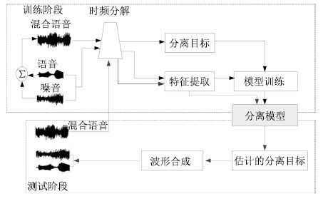
图 1给出了语音分离的一般性结构框图,主要分为5个模块: 1) 时频分解,通过信号处理的方法(听觉滤波器组或者短时傅里叶变换)将输入的时域信号分解成二维的时频信号表示.2) 特征提取,提取帧级别或者时频单元级别的听觉特征,比如,短时傅里叶变换谱(FFT-magnitude)、短时傅里叶变换对数谱(FFT-log)、Amplitude modulation spectrogram (AMS)、Relative spectral transform and perceptual linear prediction (RASTA-PLP)、Mel-frequency cepstral coefficients (MFCC)、Pitch-based features以及Multi-resolution cochleagram (MRCG). 3) 分离目标,利用估计的分离目标以及混合信号合成目标语音的波形信号.针对语音分离的不同应用特点,例如针对语音识别,语音分离在分离语音的过程中侧重减少语音畸变和尽可能地保留语音成分.针对语音通讯,语音分离侧重于提高分离语音的可懂度和感知质量.常用的语音分离目标主要分为时频掩蔽的目标、目标语音幅度谱估计的目标和隐式时频掩蔽目标,时频掩蔽目标训练一个模型来估计一个理想时频掩蔽,使得估计的掩蔽和理想掩蔽尽可能相似;目标语音幅度谱估计的方法训练一个模型来估计目标语音的幅度谱,使得估计的幅度谱与目标语音的幅度谱尽可能相似;隐式时频掩蔽目标将时频掩蔽技术融合到实际应用的模型中,用来增强语音特征或估计目标语音,隐式掩蔽并不直接估计理想掩蔽,而是作为中间的一个计算过程来得到最终学习的目标,隐式掩蔽作为一个确定性的计算过程,并没有参数需要学习,最终的目标误差通过隐式掩蔽的传导来更新模型参数. 4) 模型训练,利用大量的输入输出训练对通过机器学习算法学习一个从带噪特征到分离目标的映射函数,应用于语音分离的学习模型大致可分为浅层模型(GMM,SVM,NMF)和深层模型(DNN,DSN,CNN,RNN,LSTM,Deep NMF). 5) 波形合成,利用估计的分离目标以及混合信号,通过逆变换(逆傅里叶变换或者逆Gammatone 滤波) 获得目标语音的波形信号.
2. 时频分解
时频分解是整个系统的前端处理模块,通过时频分解,输入的一维时域信号能够被分解成二维的时频信号.常用的时频分解方法包括短时傅里叶变换[24]和Gammatone听觉滤波模型[25].
假设w(t)=w(-t)是一个实对称窗函数,X(t,f)是一维时域信号x(k)在第t时间帧、第f个频段的短时傅里叶变换系数,则
$X(t,f)=\int_{-\infty }^{+\infty }{x(k)w(k-t)\exp (-j2\pi fk)dk}$
(1) 对应的傅里叶能量幅度谱px(t,f)为
${{p}_{x}}(t,f)=\left| X(t,f) \right|$
(2) 其中, $|\cdot |$ 表示复数域的取模操作. 为了简化符号表示,用向量 $p\in R_{+}^{F\times 1}$ 表示时间帧为t的幅度谱,这里F是傅里叶变换的频带数.短时傅里叶变换是完备而稳定的[54],可以通过短时傅里叶逆变换(Inverse short-time Fourier transform,ISTFT)从X(t,f)精确重构x(k). 也就是说,可以通过估计目标语音的短时傅里叶变换系数来实现语音的分离或者增强,用 ${{\hat{Y}}_{s}}(t,f)$ 来表示估计的目标语音的短时傅里叶变换系数,那么目标语音的波形 $\hat{s}(k)$ 可以通过ISTFT计算
$\hat{s}(k)=\int_{-\infty }^{+\infty }{\int_{-\infty }^{+\infty }{{{{\hat{Y}}}_{s}}(k)w(k-t)\exp (j2\pi fk)dfdk}}$
(3) 如果不考虑相位的影响,语音分离过程可以转换为目标语音幅度谱的估计问题,一旦估计出目标语音的幅度谱 ${{\widehat{y}}_{s}}\in R_{+}^{F\times 1}$ ,联合混合语音的相位,通过ISTFT,能得到目标语音的估计波形Ŝ(k)[17].
Gammatone听觉滤波使用一组听觉滤波器g(t)对输入信号进行滤波,得到一组滤波输出G(k,f). 滤波器组的冲击响应为
$g(t)=\left\{ \begin{array}{*{35}{l}} {{t}^{l-1}}\exp (-2\pi bt)\cos (2\pi ft), & \ t\ge 0 \\ 0,& 其他 \\ \end{array} \right.$
(4) 其中,滤波器阶数l=4,b为等效矩形带宽(Equivalent rectangle bandwidth,ERB),f为滤波器的中心频率,Gammatone滤波器组的中心频率沿对数频率轴等间隔地分布在[80Hz,5kHz]. 等效矩形带宽与中心频率一般满足式(5) ,可以看出随着中心频率的增加,滤波器带宽加宽.
$ERB(f)=24.7(0.0043f+1.0) $
(5) 对于4阶的Gammatone滤波器,Patterson等[25]给出了带宽的计算公式
$b=1.093ERB(f)$
(6) 然后,采用交叠分段的方法,以20ms为帧长,10ms为偏移量对每一个频率通道的滤波响应做分帧加窗处理.得到输入信号的时频域表示,即时频单元. 在计算听觉场景分析系统中,时频单元被认为是处理的最小单位,用T-F表示.通过计算时频单元内的内毛细胞输出(或者听觉滤波器输出) 能量,就得到了听觉谱(Cochleagram) ,本文用GF(t,f)表示时间帧t频率为f的时频单元T-F的听觉能量.
3. 特征
语音分离能够被表达成一个学习问题,对于机器学习问题,特征提取是至关重要的步骤,提取好的特征能够极大地提高语音分离的性能.从特征提取的基本单位来看,主要分为时频单元级别的特征和帧级别的特征.时频单元级别的特征是从一个时频单元的信号中提取特征,这种级别的特征粒度更细,能够关注到更加微小的细节,但是缺乏对语音的全局性和整体性的描述,无法获取到语音的时空结构和时序相关性,另外,一个时频单元的信号,很难表征可感知的语音特性(例如,音素).时频单元级别的特征主要用于早期以时频单元为建模单元的语音分离系统中,例如,文献[1, 26, 30-32],这些系统孤立地看待每个时频单元,在每一个频带上训练二值分类器,判断每一个频带上的时频单元被语音主导还是被噪音主导;帧级别的特征是从一帧信号中提取的,这种级别的特征粒度更大,能够抓住语音的时空结构,特别是语音的频带相关性,具有更好的全局性和整体性,具有明显的语音感知特性.帧级别的特征主要用于以帧为建模单元的语音分离系统中,这些系统一般输入几帧上下文帧级别特征,直接预测整帧的分离目标,例如,文献[17-20, 27, 35]. 近年来,随着语音分离研究的深入,已有许多听觉特征被提出并应用到语音分离中,取得了很好的分离性能.下面,我们简要地总结几种常用的听觉特征.
1) 梅尔倒谱系数 (Mel-frequency cepstral coefficient,MFCC).为了计算MFCC,输入信号进行20ms帧长和10ms帧移的分帧操作,然后使用一个汉明窗进行加窗处理,利用STFT计算能量谱,再将能量谱转化到梅尔域,最后,经过对数操作和离散余弦变换(Discrete cosine transform,DCT)并联合一阶和二阶差分特征得到39维的MFCC.
2) PLP (Perceptual linear prediction).PLP能够尽可能消除说话人的差异而保留重要的共振峰结构,一般认为是与语音内容相关的特征,被广泛应用到语音识别中.和语音识别一样,我们使用12阶的线性预测模型,得到13维的PLP特征.
3) RASTA-PLP (Relative spectral transform PLP).RASTA-PLP引入了RASTA滤波到PLP[55],相对于PLP特征,RASTA-PLP对噪音更加鲁棒,常用于鲁棒性语音识别. 和PLP一样,我们计算13维的RASTA-PLP特征.
4) GFCC (Gammatone frequency cepstral coefficient).GFCC特征是通过Gammatone听觉滤波得到的.我们对每一个Gammatone滤波输出按照100Hz的采样频率进行采样.得到的采样通过立方根操作进行幅度压制. 最后,通过DCT得到GFCC.根据文献[56]的建议,一般提取31维的GFCC特征.
5) GF (Gammatone feature). GF特征的提取方法和GFCC类似,只是不需要DCT步骤. 一般提取64维的GF特征.
6) AMS (Amplitude modulation spectrogram). 为了计算AMS特征,输入信号进行半波整流,然后进行四分之一抽样,抽样后的信号按照32ms帧长和10ms帧移进行分帧,通过汉明窗加窗处理,利用STFT得到信号的二维表示,并计算STFT幅度谱,最后利用15个中心频率均匀分布在15.6~400Hz 的三角窗,得到15维的AMS特征.
7) 基于基音的特征 (Pitch-based feature).基于基音的特征是时频单元级别的特征,需要对每一个时频单元计算基音特征.这些特征包含时频单元被目标语音主导的可能性.我们计算输入信号的Cochleagram,然后对每一个时频单元计算6维的基音特征,详细的计算方法可以参考文献[26, 57].
8) MRCG (Multi-resolution cochleagram).MRCG的提取是基于语音信号的Cochleagram表示的. 通过Gammatone滤波和加窗分帧处理,我们能得到语音信号的Cochleagram表示,然后通过以下步骤可以计算MRCG.
步骤 1. 给定输入信号,计算64通道的Cochle- agram,CG1,对每一个时频单元取对数操作.
步骤 2. 同样地,用200ms的帧长和10ms的帧移计算CG2.
步骤 3. 使用一个长为11时间帧和宽为11频带的方形窗对CG1进行平滑,得到CG3.
步骤 4. 和CG3的计算类似,使用23 ×23的方形窗对CG1进行平滑,得到CG4.
步骤 5. 串联CG1,CG2,CG3 和 CG4得到一个64 ×4的向量,即为MRCG.
MRCG是一种多分辨率的特征,既有关注细节的高分辨率特征,又有把握全局性的低分辨率特征.
9) 傅里叶幅度谱(FFT-magnitude). 输入的时域信号进行分帧处理,然后对每帧信号进行STFT,得到STFT系数,然后对STFT进行取模操作即得到STFT幅度谱.
10) 傅里叶对数幅度谱(FFT-log-magnitude).STFT对数幅度谱是在STFT幅度谱的基础上取对数操作得到的,主要目的是凸显信号中的高频成分.
以上介绍的听觉特征是语音分离的主要特征,这些特征之间既存在互补性又存在冗余性. 研究显示,对于单个独立特征,GFCC和RASTA-PLP分别是噪音匹配条件和噪音不匹配条件下的最好特征[26].基音反映了语音的固有属性,基于基音的特征对语音分离具有重要作用,很多研究显示基于基音的特征和其他特征进行组合都会显著地提高语音分离的性能,而且基于基音的特征非常鲁棒,对于不匹配的听觉条件具有很好的泛化性能.然而,在噪音条件下,准确地估计语音的基音是非常困难,又因为缺乏谐波结构,基于基音的特征仅能用于浊音段的语音分离,而无法处理清音段,因此在实际应用中,基于基音的特征很少应用到语音分离中[26],实际上,语音分离和基音提取是一个"鸡生蛋,蛋生鸡"的问题,它们之间相互促进而又相互依赖. 针对这一问题,Zhang等巧妙地将基音提取和语音分离融合到深度堆叠网络(Deep stacking network,DSN) 中,同时提高了语音分离和基音提取的性能 [34].相对于基音特征,AMS 同时具有清音和浊音的特性,能够同时用于浊音段和清音段的语音分离,然而,AMS的泛化性能较差[58]. 针对各个特征之间的不同特性,Wang等利用Group Lasso的特征选择方法得到{AMS} +{RASTA} -{PLP} + {MFCC}的最优特征组合[26],这个组合特征在各种测试条件下取得了稳定的语音分离性能而且显著地优于单独的特征,成为早期语音分离系统最常用的特征. 在低信噪比条件下,特征提取对于语音分离至关重要,相对于其他特征或者组合特征,Chen等提取的多分辨率特征MRCG表现了明显的优势[27],逐渐取代{AMS}+ {RASTA} - {PLP} + {MFCC}的组合特征成为语音分离最常用的特征之一. 在傅里叶变换域条件下,FFT-magnitude或FFT-log-magnitude是最常用的语音分离特征,由于高频能量较小,相对于FFT-magnitude,FFT-log-magnitude能够凸显高频成分,但是,一些研究表明,在语音分离中,FFT-magnitude要略好于FFT-log-magnitude[28].
语音分离发展到现阶段,MRCG和FFT-magnitude分别成为Gammtone域和傅里叶变换域下最主流的语音分离特征.此外,为了抓住信号中的短时变化特征,一般还会计算特征的一阶差分和二阶差分,同时,为了抓住更多的信息,通常输入特征会扩展上下文帧. Chen等还提出使用ARMA模型(Auto-regressive and moving average model)对特征进行平滑处理,来进一步提高语音分离性能[27].
4. 目标
语音分离有许多重要的应用,总结起来主要有两个方面: 1) 以人耳作为目标受体,提高人耳对带噪语音的可懂度和感知质量,比如应用于语音通讯; 2) 以机器作为目标受体,提高机器对带噪语音的识别准确率,例如应用于语音识别.对于这两个主要的语音分离目标,它们存在许多密切的联系,例如,以提高带噪语音的可懂度和感知质量为目标的语音分离系统通常可以作为语音识别的前端处理模块,能够显著地提高语音识别的性能[59],Weninger等指出语音分离系统的信号失真比(Signal-to-distortion ratio,SDR)和语音识别的字错误率(Word error rate,WER)有明显的相关性[5],Weng等将多说话人分离应用于语音识别中也显著地提高了识别性能[6].尽管如此,它们之间仍然存在许多差别,以提高语音的可懂度和感知质量为目标的语音分离系统侧重于去除混合语音中的噪音成分,往往会导致比较严重的语音畸变,而以提高语音识别准确率为目标的语音分离系统更多地关注语音成分,在语音分离过程中尽可能保留语音成分,避免语音畸变.针对语音分离两个主要目标,许多具体的学习目标被提出,常用的分离目标大致可以分为三类: 时频掩蔽、 语音幅度谱估计和隐式时频掩蔽.其中时频掩蔽和语音幅度谱估计的目标被证明能显著地抑制噪音,提高语音的可懂度和感知质量[17-18].而隐式时频掩蔽通常将掩蔽技术融入到实际应用模型中,时频掩蔽作为中间处理过程来提高其他目标的性能,例如语音识别[5, 60]、目标语音波形的估计[21].
4.1 时频掩蔽
时频掩蔽是语音分离的常用目标,常见的时频掩蔽有理想二值掩蔽和理想浮值掩蔽,它们能显著地提高分离语音的可懂度和感知质量.一旦估计出了时频掩蔽目标,如果不考虑相位信息,通过逆变换技术即可合成目标语音的时域波形. 但是,最近的一些研究显示,相位信息对于提高语音的感知质量具有重要的作用[50]. 为此,一些考虑相位信息的时频掩蔽目标被相继提出,例如复数域的浮值掩蔽(Complex ideal ratio mask,CIRM)[53].
1) 理想二值掩蔽(Ideal binary mask,IBM).理想二值掩蔽(IBM)是计算听觉场景分析的主要计算目标[61],已经被证明能够极大地提高分离语音的可懂度[44-47, 62].IBM是一个二值的时频掩蔽矩阵,通过纯净的语音和噪音计算得到.对于每一个时频单元,如果局部信噪比SNR(t,f)大于某一局部阈值(Local criterion,LC),掩蔽矩阵中对应的元素标记为1,否则标记为0. 具体来讲,IBM的定义如下:
$IBM(t,f)=\left\{ \begin{array}{*{35}{l}} 1,& \text{若}SNR(t,f)>LC \\ 0,& \text{其他} \\ \end{array} \right.$
(7) 其中,SNR(t,f)定义了时间帧为t和频率为f的时频单元的局部信噪比.LC的选择对语音的可懂度具有重大的影响[63],一般设置LC小于混合语音信噪比5dB,这样做的目的是为了保留足够多的语音信息. 例如,混合语音信噪比是-5dB,则对应的LC设置为-10dB.
2) 目标二值掩蔽(Target binary mask,TBM). 类似于IBM,目标二值掩蔽(TBM)也是一个二值的时频掩蔽矩阵. 不同的是,TBM是通过纯净语音的能量和一个固定的参照噪音(Speech-shaped noise,SSN) 的能量计算得到的. 也就是说,在式(7) 中的SNR(t,f)项是用参考的SSN而不是实际的噪音计算的.尽管TBM的计算独立于噪音,但是实验测试显示TBM取得了和IBM相似的可懂度提高[63].TBM能够提高语音的可懂度的原因是它保留了与语音感知密切相关的时空结构模式,即语音能量在时频域上的分布. 相对于IBM,TBM可能更加容易学习.
3) Gammtone域的理想浮值掩蔽(Gammtone ideal ratio mask,IRM_Gamm)
理想浮值掩蔽定义如下:
$\begin{align} & IR{{M}_{gamm}}(t,f)\text{=}{{\left( \frac{{{S}^{2}}(t,f)}{{{S}^{2}}(t,f)+{{N}^{2}}(t,f)} \right)}^{\beta }}\text{=} \\ & {{\left( \frac{SNR(t,f)}{SNR(t,f)+1} \right)}^{\beta }} \\ \end{align}$
(8) 其中,S2(t,f)和N2(t,f)分别定义了混合语音中时间帧为t和频率为f的时频单元的语音和噪音的能量.β是一个可调节的尺度因子. 如果假定语音和噪音是不相关的,那么IRM在形式上和维纳滤波密切相关[9, 64].大量的实验表明β = 0.5是最好的选择,此时,式(8) 和均方维纳滤波器非常相似,而维纳滤波是最优的能量谱评估[9].
4) 傅里叶变换域的理想浮值掩蔽(FFT ideal ratio mask,IRM_FFT).类似于Gammtone域的理想浮值掩蔽,傅里叶域的理想浮值掩蔽IRM_FFT的定义如下:
$\begin{align} & IR{{M}_{FFT}}(t,f)\text{=}\frac{{{\left| {{Y}_{s}}(t,f) \right|}^{2}}}{{{\left| {{Y}_{s}}(t,f) \right|}^{2}}+{{\left| {{Y}_{n}}(t,f) \right|}^{2}}}\text{=} \\ & \frac{{{P}_{s}}(t,f)}{{{P}_{s}}(t,f)+{{P}_{n}}(t,f)} \\ \end{align}$
(9) 其中,Ys(t,f)和Yn(t,f)是混合语音中纯净的语音和噪音的短时傅里叶变换系数.Ps(t,f)和Pn(t,f)分别是它们对应的能量密度.
5) 短时傅里叶变换掩蔽(Short-time Fourier transform mask,FFT-Mask).不同于IRM_FFT,FFT-Mask的定义如下:
$Mas{{k}_{FFT}}(t,f)=\frac{\left| {{Y}_{s}}(t,f) \right|}{\left| X(t,f) \right|}$
(10) 其中,Ys(t,f)和X(t,f)是纯净的语音和混合语音的短时傅里叶变换系数.IRM_FFT的取值范围在[0,1],显然FFT-Mask的取值范围可以超过1.
6) 最优浮值掩蔽(Optimal ratio time-frequency mask,ORM).理想浮值掩蔽(IRM) 是假定在语音和噪音不相关的条件下,能够取得最小均方误差意义下最大信噪比增益[42-43].然而在真实环境中,语音和噪音通常存在一定的相关性,针对这个问题,Liang等[42-43]推导出一般意义下的最小均方误差的最优浮值掩蔽,定义如下:
$\begin{align} & ORM(t,f)= \\ & \frac{{{P}_{s}}(t,f)+\Re ({{Y}_{s}}(t,f)Y_{n}^{*}(t,f))}{{{P}_{s}}(t,f)+{{P}_{n}}(t,f)+2\Re ({{Y}_{s}}(t,f)Y_{n}^{*}(t,f))} \\ \end{align}$
(11) 其中, $\Re (\cdot )$ 表示取复数的实部,*表示共轭操作.相对于IRM,ORM考虑了语音和噪音的相关性,其变化范围更大,估计难度也更大.
7) 复数域的理想浮值掩蔽(Complex ideal ratio mask,CIRM).传统的IRM定义在幅度域,而CIRM定义在复数域.其目标是通过将CIRM作用到带噪语音的STFT系数得到目标语音的STFT系数.具体地,给定带噪语音在时间帧为t和频率为f的时频单元的STFT系数X,那么目标语音在对应时频单元的STFT系数Y可以通过下式计算得到:
$Y=M\times X$
(12) 其中,×定义复数乘法操作,M定义时间帧为t和频率为f的时频单元的CIRM.通过数学推导我们能计算得到:
$M=\frac{{{X}_{r}}{{Y}_{r}}+{{X}_{i}}{{Y}_{i}}}{X_{r}^{2}+X_{i}^{2}}+j\frac{{{X}_{r}}{{Y}_{i}}-{{X}_{i}}{{Y}_{r}}}{X_{r}^{2}+X_{i}^{2}}$
(13) 其中,Xr和Yr分别是X和Y的实部,Xi和Yi分别是X和Y的虚部,j是虚数单位.定义Mr和Mi分别是M的实部和虚部,那么,
${{M}_{r}}=\frac{{{X}_{r}}{{Y}_{r}}+{{X}_{i}}{{Y}_{i}}}{X_{r}^{2}+X_{i}^{2}}$
(14) ${{M}_{i}}=\frac{{{X}_{r}}{{Y}_{i}}-{{X}_{i}}{{Y}_{r}}}{X_{r}^{2}+X_{i}^{2}}$
(15) 在实际语音分离中通常不会直接估计复数域的M,而是通过估计其实部Mr和虚部Mi.但Mr和Mi的取值可能会超过[0,1],这往往会增大Mr和Mi估计难度. 因此,在实际应用中通常会利用双曲正切函数对Mr和Mi进行幅度压制.
4.2 语音幅度谱估计
如果不考虑相位的影响,语音分离问题可以转化为目标语音幅度谱的评估,一旦从混合语音中评估出了目标语音的幅度谱,利用混合语音的相位信息,通过逆变换即可得到目标语音的波形.常见的幅度谱包括Gammtone域幅度谱和STFT幅度谱.
1) Gammtone域幅度谱 (Gammatone frequency power spectrum,GF-POW).时域信号经过Gammtone滤波器组滤波和分帧加窗处理,可以得到二维的时频表示Cochleagram.直接估计目标语音的Gammtone域幅度谱(GF-POW)能够实现语音的分离.对于Gammtone滤波,由于没有直接的逆变换方法,我们可以通过估计的GF-POW和混合语音的GF-POW构造一个时频掩蔽 $\sqrt{S_{GF}^{2}(t,f)/X_{GF}^{2}(t,f)}$ 来合成目标语音的波形,其中, $S_{GF}^{2}(t,f)$ 和 $X_{GF}^{2}(t,f)$ 分别是纯净语音和混合语音在Gammtone域下时间帧为t和频带为f的时频单元的能量.
2) 短时傅里叶变换幅度谱 (Short-time Fourier transform spectral magnitude,FFT-magnitude). 时域信号经过分帧加窗处理,然后通过STFT,可以得到二维的时频表示,如果不考虑相位的影响,我们可以直接估计目标语音的STFT幅度谱,利用原始混合语音的相位,通过IFTST可以估计得到目标语音的时域波形.
4.3 隐式时频掩蔽
语音分离旨在从混合语音中分离出语音成分,尽管可以通过估计理想时频掩蔽来分离目标语音,但理想时频掩蔽是一个中间目标,并没有针对实际的语音分离应用直接优化最终的实际目标. 针对这些问题,隐式时频掩蔽被提取,在这些方法中,时频掩蔽作为一个确定性的计算过程被融入到具体应用模型中,例如识别模型或者分离模型,它们并没有估计理想时频掩蔽,其最终的目标是估计目标语音的幅度谱甚至是波形,或者提高语音识别的准确率.
Huang等提出将掩蔽融合到目标语音的幅度谱估计中[19, 28].在文献[29]中,深度神经网络作为语音分离模型,时频掩蔽函数作为额外的处理层加入到网络的原始输出层,如图 2所示,通过时频掩蔽,目标语音的幅度谱从混合语音的幅度谱中估计出来.其中时频掩蔽函数Ms和Mn通过神经网络原始输出(语音和噪音幅度谱的初步估计)计算得到的,如下:
${{M}_{s}}=\frac{\left| {{\widehat{y}}_{s}} \right|}{\left| {{\widehat{y}}_{s}} \right|+\left| {{\widehat{y}}_{n}} \right|},{{M}_{n}}=\frac{\left| {{\widehat{y}}_{n}} \right|}{\left| {{\widehat{y}}_{s}} \right|+\left| {{\widehat{y}}_{n}} \right|}$
(16) 
一旦时频掩蔽被计算出来,就可以通过掩蔽技术从混合语音的幅度谱{X}估计出语音和噪音的幅度谱 ${{\widetilde{y}}_{s}}$ 和 ${{\widetilde{y}}_{n}}$ :
${{\widetilde{y}}_{s}}={{M}_{s}}\otimes X,\ {{\widetilde{y}}_{n}}={{M}_{n}}\otimes X$
(17) 需要注意的是原始的网络输出并不用来计算误差函数,仅仅用来计算时频掩蔽函数,时频掩蔽函数是确定性的,并没有连接权重,掩蔽输出用来计算误差并以此来更新模型参数.
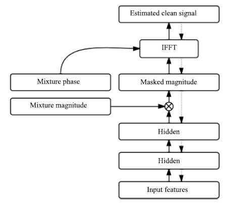
Wang等提出将时频掩蔽融合到目标语音波形估计中[21],在文献[21]中,时频掩蔽作为神经网络的一部分,掩蔽函数从混合语音的STFT幅度谱估计目标语音的STFT幅度谱,然后通过ISTFT,利用混合语音的相位信息和估计的STFT幅度谱合成目标语音的时域波形,如图 3所示,估计的时域波形与目标波形计算误差,最后通过反向传播更新网络权重.假设m是最后一个隐层的输出,它可以看成是估计的掩蔽,用来从混合语音的STFT幅度谱x中估计目标语音的STFT幅度谱 ${{\widetilde{y}}_{s}}$ .
${{\widetilde{y}}_{s}}=m\otimes x$
(18) 评估的目标语音幅度谱加上对应的混合语音的相位p输入到逆傅里叶变换层能够得到目标语音的时域波形信号.
$\widehat{s}=\operatorname{IFFT}({{[c,\operatorname{flipud}({{({{c}_{2:d}})}^{*}})]}^{T}})$
(19) 其中,c是目标语音的傅里叶变换系数,它能够通过下面的公式得到:
$c={{\widetilde{y}}_{s}}\otimes {{e}^{jp}}$
(20) d = F/2,F是傅里叶变换的分析窗长.flipud定义了向量的上下翻转操作,*是复数的共轭操作.下标m:n取向量从m到n的元素的操作.
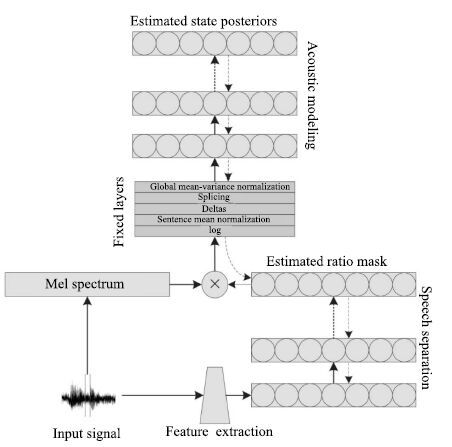
Narayanan等[60]提出将时频掩蔽融入到语音识别的声学模型中,时频掩蔽作为神经网络的中间处理层,从带噪的梅尔谱特征中掩蔽出语音的梅尔谱特征,然后输入到下层网络中进行状态概率估计,如图 4 所示.注意时频掩蔽仅仅是神经网络的中间处理层的输出,并不是以理想时频掩蔽作为目标学习而来的,确切地说是根据语音识别的状态目标学习而来的,实验结果显示,时频掩蔽输出具有明显的降噪效果,这从侧面显示了语音识别与语音分离之间存在密切联系.
以上介绍的是监督性语音分离的主要目标. 在时频掩蔽目标中,理想二值掩蔽具有最为简单的形式,而且具有听觉感知掩蔽的心理学依据,是早期监督性语音分离最常用的分离目标,其分离的语音能够极大地提高语音的可懂度,然而语音的听觉感知质量往往得不到提高.理想浮值掩蔽具有0到1的平滑形式,近似于维纳滤波,不仅能够提高分离语音的可懂度而且能够显著地提高语音的感知质量,在语音和噪音独立的情况下能够取得最优信噪比增益. 相比于理想二值掩蔽,最优浮值掩蔽是更为一般意义下的最优信噪比增益目标,它考虑了语音和噪音之间的相关性,但是最优浮值掩蔽的学习难度也相对较大,目前尚未应用到监督性语音分离中. 之前大部分时频掩蔽,都没有考虑语音的相位信息,而研究表明相位信息对于提高语音的感知质量具有重要作用.复数域的理想浮值掩蔽考虑了语音的相位信息,被应用到监督性语音分离中,取得了显著的性能提高. 语音幅度谱估计的目标直接估计目标语音的幅度谱,相对于时频掩蔽目标,更为直接也更为灵活,然而其学习难度也更大,常用的语音幅度谱估计的目标是短时傅里叶变换域的语音幅度谱.隐式时频掩蔽目标并没有直接估计理想时频掩蔽,而是将时频掩蔽融入到实际应用的模型中,直接估计最终的目标,例如目标语音的波形或者语音识别的状态概率,这种方式学习到的时频掩蔽和实际目标最相关,目前,正广泛应用于语音分离系统中.
5. 模型
语音分离能够很自然地表达成一个监督性学习问题,一个典型的监督性语音分离系统利用学习模型学习一个从带噪特征到分离目标的映射函数.目前已有许多学习模型应用到语音分离中,常用的模型大致可以分为两类:浅层模型和深层模型. 在早期的监督性语音分离中[1, 14, 31],浅层模型通常直接对输入的带噪时频单元的分布进行概率建模或区分性建模,例如GMM[1]和SVM[31],或者直接对输入的带噪特征数据进行矩阵分解,以推断混合数据中语音和噪音的成分,例如NMF[14].由于浅层模型没有从数据中自动抽取有用特征的能力,因此,它们严重依赖于人工设计的特征,另外,浅层模型对高维数据处理的能力通常比较有限,很难通过扩展上下文帧来挖掘语音信号中的时频相关性.深层模型是近几年来受到极大关注的学习模型,在语音和图像等领域都取得了巨大的成功.由于深层模型层次化的非线性处理,使得它能够自动抽取输入数据中对目标最有力的特征表示,相比于浅层模型,深层模型能够处理更原始的高维数据,对特征设计的知识要求相对较低,而且深层模型擅长于挖掘数据中的结构化特性和结构化输出预测.由于语音的产生机制,语音分离的输入特征和输出目标都呈现了明显的时空结构,这些特性非常适合用深层模型来进行建模.许多深层模型广泛应用到语音分离中,包括DNN[18]、 DSN[33-34]、 CNN[22]、 RNN[19-20, 28]、 Deep NMF[23] 和 LSTM[39].
5.1 浅层模型
1) 高斯混合模型(GMM). 高斯混合模型能够刻画任意复杂的分布,Kim等[1]利用GMM分别对每一个频带被目标语音主导的时频单元和被噪音主导的时频单元进行建模,这里各个频带是独立建模的,在测试阶段,给定时频单元的输入特征,计算被目标语音主导和被噪音主导的概率,然后进行贝叶斯推断,判断时频单元是被目标语音主导还是被噪音主导,如果被语音主导标记为1,否则标记为0,当所有的时频单元被判断出来,则二值掩蔽被估计出来. 最后,利用估计的二值掩蔽和混合语音的Gammtone滤波输出合成目标语音的时域波形.
高斯混合模型是一种生成式的模型,目标语音主导的时频单元的概率分布和噪音主导的时频单元的概率分布有很多重叠部分,并且它不能挖掘特征中的区分信息,不能进行区分性训练.孤立地对每一个频带建模,无法利用频带间的相关性,同时会导致训练和测试代价过大,很难具有实用性.
2) 支持向量机(SVM). 支持向量机能够学习数据中的最优分类面,以区分不同类别的数据.Han等[32]提出用SVM对每一个频带的时频单元进行建模,学习被目标语音主导的时频单元和被噪音主导的时频单元最优区分面.在测试阶段,输入时频单元的特征,通过计算到分类面的距离实现时频单元的分类.
相比于GMM,SVM取得了更好的分类准确性和泛化性能.这主要得益于SVM的区分性训练.但是SVM仍然是对每一个时频单元进行单独建模,忽略了它们之间的相关性和语音的时空结构特性,同时SVM是浅层模型,并没有特征抽象和层次化学习的能力.
3) 非负矩阵分解(NMF). 非负矩阵分解是著名的表示学习方法,它能挖掘隐含在非负数据中的局部表示. 给定非负矩阵 $X\in {{R}_{+}}$ ,非负矩阵分解将X 近似分解成两个非负矩阵的乘积, $X\approx WH$ ,其中W是非负基矩阵,H是对应的激活系数矩阵.当非负矩阵分解应用到纯净语音或者噪音的幅度谱时,NMF能挖掘出语音或者噪音的基本谱模式. 在语音分离中,首先在训练阶段,在纯净的语音和噪音上分别训练NMF模型,得到语音和噪音的基矩阵. 然后,在测试阶段,联合语音和噪音的基矩阵得到一个既包含语音成分又包含噪音成分的更大的基矩阵,利用得到的基矩阵,通过非负线性组合重构混合语音幅度谱,当重构误差收敛时,语音基和噪音基对应的激活矩阵被计算出来,然后利用非负线性组合即可分离出混合语音中的语音和噪音.
NMF是单层线性模型,很难刻画语音数据中的非线性关系,另外,在语音分离过程中,NMF的推断过程非常费时,很难达到实时性要求,大大限制了NMF在语音分离中的实际应用.
5.2 深层模型
1) 深度神经网络(DNN). DNN是最常见的深层模型,一个典型的DNN通常由一个输入层,若干个非线性隐含层和一个输出层组成,各个层依次堆叠,上层的输出输入到下一层中,形成一个深度的网络.层次化的非线性处理使得DNN具有强大的表示学习的能力,能够从原始数据中自动学习对目标最有用的特征表示,抓住数据中的时空结构. 然而,深度网络的多个非线性隐含层使得它的优化非常困难,往往陷入性能较差的局部最优点. 为解决这个问题,2006年Hinton等提出了一种无监督的预训练方式,极大地改善了深度神经网络的优化问题[65]. 自此,深度神经网络得到广泛的研究,在语音和图像等领域取得巨大的成功.Xu等将DNN应用于语音分离中,取得了显著的性能提升. 在文献[18]中,DNN被用来学习一个从带噪特征到目标语音的对数能量幅度谱的映射函数,如图 5所示. 上下文帧的对数幅度谱作为输入特征,通过两个隐层的非线性变换和输出层的线性变换,估计得到对应帧的目标语音的对数幅度谱. 最后,使用混合语音的相位,利用ISTFT得到目标语音的时域波形信号.
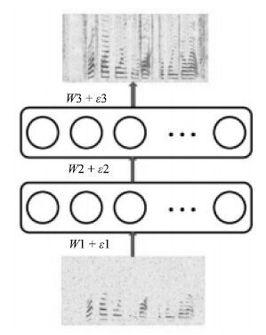
实验结果显示Xu等提出的方法在大规模训练数据上取得了优异的语音分离性能.然而,直接估计目标语音的对数幅度谱是一个非常困难的任务,需要大量的训练数据才能有效地训练模型,同时其泛化性能也是一个重要的问题.
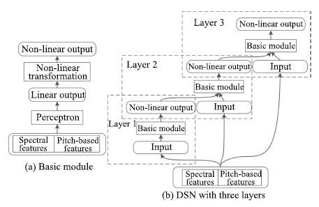
2) 深度堆叠网络(DSN). 语音信号具有很强的时序相关性,探究这些特性能够提高语音分离的性能,为此,Nie等[33]利用DSN的层次化模块结构对时频单元的时序相关性进行建模,定义为DSN-TS,如图 6所示. DSN的基本模块是一个由一个输入层,一个隐层和一个线性输出层组成的前向传播网络. 模块之间相互堆叠,每一个模块依次对应一个时刻帧,前一个模块的输出连接上下一个时刻的输入特征作为下一个模块的输入,如此类推,便可估计所有时刻的时频单元的掩蔽.

相比于之前的模型,DSN-TS考虑了时频单元之间的时序关系,在分离性能上取得进一步提高.然而,DSN-TS对每一个频带单独建模,忽略了频带之间的相关性.
基音是语音的一个显著的特征,在传统的计算听觉场景分析中常被用作语音分离的组织线索.基于基音的特征也常被用于语音分离,然而,噪音环境下,基音的提取是一个挑战性的工作,Zhang等[34]巧妙地将噪声环境下的基音提取和语音分离融合到DSN中,定义为DSN-Pitch,如图 7所示. 在DSN-Pitch中,基音提取和语音分离交替进行,相互促进.DSN-Pitch同时提高了语音分离的性能和基音提取的准确性,然而,DSN-Pitch依然对每一个时频单元单独建模,严重忽略了它们之间的时空相关性.
3) 深度循环神经网络(Deep recurrent neural network,DRNN).由于语音的产生机制,语音具有明显的长短时谱依赖性,这些特性能够被用来帮助语音分离. 尽管DNN具有强大的学习能力,但是DNN仅能通过上下文或者差分特征对数据中的时序相关性进行有限的建模,而且会极大地增加输入数据的维度,大大地增加了学习的难度.RNN是非常常用的时序模型,利用其循环连接能够对时序数据中长短时依赖性进行建模.Huang等将RNN应用到语音分离中,取得比较好的语音分离性能[29].标准的RNN仅有一个隐层,为了对语音数据进行层次化抽象,Huang等[29]使用深度的RNN作为最终的分离模型,如图 8所示.
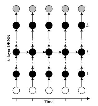
相对于DNN,DRNN能够抓住数据中时序相关性,但是由于梯度消失的问题,DRNN不容易训练,对长时依赖的建模能力有限. 实验结果表明,相对于DNN,DRNN在语音分离中的性能提升比较有限.
4) 长短时记忆网络(Long short-term memory,LSTM). 作为RNN的升级版本,在网络结构上,LSTM增加了记忆单元、输入门、遗忘门和输出门,这些结构单元使得LSTM相比于RNN在时序建模能力上得到巨大的提升,能够记忆更多的信息,并能有效抓住数据中的长时依赖.语音信号具有明显的长短时依赖性,Weninger等将LSTM应用到语音分离中,取得了显著的性能提升[5, 39].
5) 卷积神经网络(Convolutional neural network,CNN).CNN在二维信号处理上具有天然的优势,其强大的建模能力在图像识别等任务已得到验证. 在语音分离中,一维时域信号经过时频分解技术变成二维的时频信号,各个时频单元在时域和频域上具有很强的相关性,呈现了明显的时空结构.CNN 擅长于挖掘输入信号中的时空结构,具有权值共享,形变鲁棒性特性,直观地看,CNN适合于语音分离任务. 目前CNN已应用到语音分离中,在相同的条件下取得了最好的分离性能,超过了基于DNN的语音分离系统[22, 66].
6) 深度非负矩阵分解(Deep nonnegative matrix factorization,Deep NMF). 尽管NMF能抓住隐含在非负数据中的局部基表示,但是,NMF是一个浅层线性模型,很难对非负数据中的结构特性进行层次化的抽象,也无法处理数据中的非线性关系.而语音数据中存在丰富的时空结构和非线性关系,挖掘这些信息能够提高语音分离的性能. 为此,Le Roux等将NMF扩展成深度结构,在语音分离应用上取得巨大的性能提升[23, 40-41].
总结以上介绍的语音分离模型,可以看到: 浅层模型,复杂度低但泛化性能好,无法自动学习数据中的特征表示,其性能严重依赖于人工设计的特征,基于浅层模型的语音分离系统其性能和实用性有限; 深度模型,复杂度高建模能力强,其泛化性能可以通过扩大训练数据量来保证,另外,深度模型能够自动学习数据中有用的特征表示,因此对特征设计的要求不高,而且,能够处理复杂的高维数据,可以通过将上下文帧级联输入到深度模型中,以便为语音分离提供更多的信息. 同时,深度模型具有丰富的结构,能够抓住语音数据的很多特性,例如时序性、时空相关性、长短时谱依赖性和自回归性等. 深度模型能够处理复杂的结构映射,因此,能够为基于深度模型的语音分离设计更加复杂的目标来提高语音分离的性能.目前,监督性语音分离的主流模型是深度模型,并开始将浅层模型扩展成深度模型.
6. 总结与展望
6.1 总结
本文从时频分解、特征、目标和模型四个方面对基于深度学习的语音分离技术的整体框架和主要流程进行综合概述和分析比较.对于时频分解,听觉滤波器组和傅里叶变换是最常用的技术,它们在分离性能上没有太大的差异. 听觉滤波器组在低频具有更高的分辨率,但是计算复杂度比较高,傅里叶变换具有快速算法而且是一个可逆变换,在监督性语音分离中日益成为主流. 对于特征,目前帧级别的MRCG和FFT-magnitude分别是Gammtone域下和傅里叶变换域下最主流的特征,已经在许多研究中得到验证,是目前语音分离使用最多的特征.时频掩蔽是监督性语音分离最主要的分离目标,浮值掩蔽在可懂度和感知质量上都优于二值掩蔽,目前是语音分离的主流目标. 然而,时频掩蔽并不能优化实际的分离目标,傅里叶幅度谱是一种更接近实际目标的分离目标,相对于时频掩蔽具有更好的灵活性,能够进行区分性学习,日益得到研究者的重视,但是,其学习难度更大.目前结合时频掩蔽和傅里叶幅度谱的隐式掩蔽目标显示了光明的研究前景,正被日益广泛地应用到语音分离中,而且各种变形的隐式掩蔽目标正不断地被提出.自从语音分离被表达成监督性学习问题,各种学习模型被尝试着应用到语音分离中,在各种模型中,深度模型在语音分离任务中显示了强大的建模能力,取得了巨大的成功,目前已经成为语音分离的主流方法.
语音分离在近几年来得到研究者的广泛关注,针对时频分解,特征、目标和模型都有许多方法被提出. 对现存的方法,我们从建模单元、分离目标和学习模型三个方面进行简单的分类总结:
1) 建模单元. 语音分离的建模单元主要有两类: a) 时频单元的建模;b) 帧级别的建模. 时频单元的建模对每一个时频单元单独建模,通过分类模型估计每一个时频单元是被语音主导还是被噪音主导,早期,基于二值分类的监督性语音分离通常是基于时频单元建模的.帧级别的建模将一帧或者若干帧语音的所有时频单元看成一个整体,同时对它们进行建模,估计的目标也是帧级别的. 相对于时频单元的建模,帧级别的建模能够抓住语音的时频相关性,一般认为帧级别的建模能取得更好的语音分离性能. 目前,帧级别的建模已成为监督性语音分离的主流建模方法,从时频单元到帧级别的建模单元转变是一个巨大的进步,这主要得益于深度学习强大的表示与学习能力,能够进行结构性输出学习.传统的浅层学习能力很难学习结构复杂的高维度的输出.
2) 分离目标. 语音分离的目标主要分为三类: a) 时频掩蔽;b) 目标语音的幅度谱估计; c) 隐式时频掩蔽.时频掩蔽是语音分离的主要目标,许多监督性语音分离系统从带噪特征中估计目标语音的二值掩蔽或者浮值掩蔽,然而,时频掩蔽是一个中间目标,并没有直接优化实际的语音分离目标.相对于时频掩蔽,估计目标语音的幅度谱更接近实际的语音分离目标,而且更为灵活,能够更充分利用语音和噪音的特性构造区分性的训练目标.但是,由于幅度谱的变化范围比较大,在学习难度上要比时频掩蔽目标的学习难度大.深度学习具有强大的学习能力,现在已有许多基于深度学习的语音分离方法直接估计目标语音的幅度谱.隐式的时频掩蔽方法将时频掩蔽融合到深度神经网路中,并不直接估计理想时频掩蔽,而是作为中间处理层帮助实际目标的估计.在这里,时频掩蔽并不是神经网络学习的目标,它是通过实际应用的目标的估计误差隐式地得到的.相对于时频掩蔽和目标语音幅度谱估计的方法,隐式时频掩蔽方法融合了时频掩蔽和目标语音幅度谱估计方法的优势,能够取得更好的语音分离性能,目前已有几个基于隐式的时频掩蔽方法的监督性语音分离方法被提出,并且取得了显著的性能提升.
3) 学习模型. 监督性语音分离的学习模型主要分为两类: a) 浅层模型;b) 深层模型. 早期的监督性语音分离主要使用浅层模型,一般对每一个频带的时频单元单独建模,并没有考虑时频单元之间的时空相关性.基于浅层模型的语音分离系统分离的语音的感知质量通常比较差.随着深度学习的兴起,深层模型开始广泛应用到语音分离中,目前已经成为监督性语音分离最主流的学习模型.深层模型具有强大的建模能力,能够挖掘数据中的深层结构,相对于浅层模型,深层模型分离的语音不仅在感知质量和可懂度方便都得到巨大的提升,而且随着数据的增大,其泛化性能和分离性能得到不断的提高.
6.2 展望
最近几年,在全世界研究者的共同努力下,监督性语音分离得到巨大的发展. 针对监督性语音分离的特征、目标和模型三个主要方面都进行了深入细致的研究,取得许多一致性的共识. 目前,监督性语音分离的框架基本成熟,即利用深度模型学习一个从带噪特征到分离目标的映射函数.很难在框架层面进行重大的改进,针对现有的框架,特别是基于深度学习的语音分离框架,我们认为,未来监督性语音分离可能在下面几个方面.
1) 泛化性. 尽管监督性语音分离取得了很好的分离性能,特别是深度学习的应用,极大地促进了监督性语音分离的发展.但在听觉条件或者训练数据不匹配的情况下,例如噪音不匹配和信噪比不匹配的情况下,分离性能会急剧下降.目前解决这个问题最有效方法是扩大数据的覆盖面,但现实情况很难做到覆盖大部分的听觉环境,同时训练数据增大又带来训练时间的增加,不利于模型更新.我们认为解决这个问题的两个可行的方向是: a) 挖掘人耳的听觉心理学知识,例如将计算听觉场景分析的知识融入到监督性语音分离模型中.人耳对于声音的处理具有很好的鲁棒性.早期计算听觉场景分析的许多研究表明基音和听觉掩蔽等对噪音是非常鲁棒的,将这些积累的人工知识和计算听觉场景分析的处理过程有效融入到监督性语音分离中可能会提高监督性语音分离的泛化性能.b) 更多地关注和挖掘语音的固有特性. 由于人声产生的机理,人声具有很多明显的特性,例如稀疏性、 时空连续性、明显的谐波结构、自回归性、长短时依赖性等,对于噪音,这些特性具有明显的区分性,而且,对于不同的人发出的人声,不同的语言和内容,人声都具有这些特性. 而噪音的变化却多种多样,很难找到共有的模式.因此应该将更多的精力放到对语音固有特性的研究和挖掘上而不是只关注噪音.将语音固有的特性融入到监督性语音分离模型中可能会提高语音分离的性能和泛化能力.
2) 生成式模型和监督性模型联合.人耳对声音的处理过程可能是模式驱动的,即在大脑高层可能存储有许多关于语音的基本模式,当我们听到带噪语音的时候,带噪语音会激发大脑中相似的语音模式响应,这些先后被激活的语音模式组合起来即可形成大脑可理解的语义单元,使得人们能从带噪语音中听清语音.而这些语音模式一方面是从父母继承而来的,一方面是后天学习来的.我们可以利用生成式模型从大量纯净的语音中学习语音的基本谱模式,然后利用监督性学习模型来估计语音基本谱模式的激活量,利用这些激活的基本谱模式可以重构纯净的语音.基本谱模式的学习可以利用很多生成式模型,而它们之间的融合也可以有多种形式,这方面有许多内容值得进一步探讨.
-
表 1 直接法与非直接法优缺点对比
Table 1 The comparison between direct methods and indirect methods
直接法 非直接法 目标函数 最小化光度值误差 最小化重投影误差 优点1 使用了图像中的所有信息 适用于图像帧间的大幅运动 优点2 使用帧间的增量计算减小了每帧的计算量 比较精确, 对于运动和结构的计算效率高 缺点1 受限于帧与帧之间的运动比较小的情况 速度慢(计算特征描述等) 缺点2 通过对运动结构密集的优化比较耗时 需要使用RANSAC等鲁棒估计方法 容易失败 场景的照明发生变化 纹理较弱的地方  下载: 导出CSV
表 2 常用运动模型先验假设
Table 2 The common used motion model assumption
运动模型假设 方法 恒速运动模型 ORB SLAM, PTAM, DPPTAM, DSO 帧位姿变化为0 DPPTAM, SVO, LSD SLAM 帧间仿射变换 DT SLAM
下载: 导出CSV
表 3 常用的鲁棒估计器
Table 3 The common used robust estimators
类型 $\rho(x)$ $\ell_2$ $\dfrac{x^2}{2}$ $\ell_1$ $|x|$ $\ell_1-\ell_2$ $2\left(\sqrt{1+\dfrac{x^2}{2}}-1\right)$ $\ell_p$ $\dfrac{|x|^\nu}{\nu}$ Huber $\begin{cases} \dfrac{x^2}{2}, &\mbox{若} \ |x|\leq c\\ c\left(|x|- \dfrac{c}{2}\right), &\mbox{若} \ |x| > c \end{cases}$ Cauchy $\dfrac{C^2}{2}\ln\left(1+\left( \dfrac{x}{c}\right)^2\right)$ Tukey $\begin{cases} \dfrac{c^2}{6}\left(1-\left[1-\left( \dfrac{x}{c}\right)^2\right]^3\right), &\mbox{若} |x|\leq c \\ \dfrac{c^2}{6}, &\mbox{若} \ |x| > c \end{cases}$ t分布 $\dfrac{\nu+1}{\nu+\left( \dfrac{r}{\sigma}\right)^2}$
下载: 导出CSV
表 4 VO系统中的鲁棒目标函数设计
Table 4 The common used robust objection function in VO systems
VO系统 目标函数框架 PTAM Tukey biweight DSO Huber DT SLAM Cauchy distribution DPPTAM Reweighted Tukey DTAM Weighted Huber norm
下载: 导出CSV
表 5 深度图模型
Table 5 The common used models of depth map
VO系统 深度模型 SVO 高斯混合均匀模型 DSO 高斯模型 DT SLAM 极线分段约束[61] DPPTAM半稠密 一致性假设 DPPTAM稠密 能量函数1 DTAM 能量函数2 LSD SLAM 能量函数3 1光度值误差+图像空间平滑+平面块假设.
2使用光度值误差和图像空间平滑(正则).
3光度值误差和关键帧间方法惩罚.
下载: 导出CSV
表 6 深度网络定位系统特点
Table 6 The comparison of the learning based localization methods
定位系统 目标函数 输入数据 输出结果 网络类型 面向的问题 LSM$^{1}$[79] SFA$^{2}$ 2帧图像 位姿 CNN 运动估计 PoseNet 位姿误差(7) RGB单帧图像 位姿 GoogLeNet$^{3}$ 重定位 3D-R2N2$^{5}$[72] 体素交叉熵$^{4}$ 单/多帧图像 图像重建 CNN + LSTM 三维重建 LST$^{6}$[74] 位姿误差 IMU 位姿 LSTM 数据融合 MatchNet 相似度交叉熵$^{7}$ 2帧图像 匹配度 CNN + FC 图像块匹配 GVNN 光度值误差 当前/参考图像 位姿 CNN + SE3$^{8}$ 视觉里程计 HomographNet 图像点误差 2帧图像 单应矩阵 CNN 估计单应矩阵 SFM-Net[80] 相机运动误差 RGBD图像 相机运动、三维点云 全卷积 相机运动估计和三维重建 SE3-Net[81] 物体运动误差 点云数据 物体运动 卷积+反卷积 刚体运动 $^{1}$ Learning to see by moving.
$^{2}$ SFA使用图像的密集像素匹配目标(损失)函数, 详见文献[82].
$^{3}$ GoogLeNet是一种22层的CNN网络, 常用于分类识别等.
$^{4}$体素是一个三维向量, 对应像素(二维), 具有三维坐标, 表示点对应的空间位置的颜色值, 详见文献[83].
$^{5}$ 3D-R2N2(3D Recurrent reconstruction neural network).
$^{6}$ Learning to fuse.
$^{7}$文章在全连接层中使用Softmax层, 因此输出为0/1值, 全连接层输入为拼接的特征点对, 目标函数为sofmax输出值的交叉熵误差.
$^{8}$除了使用SE3层, 还有包括投影层, 反投影层等.
下载: 导出CSV
表 8 VO系统常用验证数据集
Table 8 The common used dataset in VO system
名称 发布时间 数据类型 相机类型 真值来源 传感器 文献 KITTI VO 2012 png 双目 GPS 激光 [103] TUM-Monocular 2012 jpg 单目 无 否 [25] TUM-RGBD 2012 png + d RGBD 无 否 [104] ICL NUM 2014 png 双目 $^{4}$ 无 [105] EuRoC MAV 2016 ROS$^{1}$ + ASL$^{2}$ 双目 VICON$^{3}$ IMU [106] Scene Flow 2016 png 双目 $^{4}$ 无 [107] COLD$^{5}$ 2009 JPEG 全向$^{6}$ 无 激光$^{7}$ [108] NYU depth 2011/2012 png + d RGBD 无 无 [109], [110] PACAL 3D + 2014 JPEG 单目 $^{4}$ 无 [111] $^1$ ROS中使用的一种bag记录文件, 使用ROS可以广播文件中的数据为消息.
$^2$ ASL为该数据集自定义格式.
$^3$除了使用VICON另外还有Laser tracker以及3D structure scan, 具体为Vicon motion capture system (6D pose), Leica MS50 laser tracker (3D position), Leica MS50 3D structure scan.
$^4$合成数据集, 存在真值.
$^5$这里有一个COLD数据的拓展数据集, 详见http://www.pronobis.pro/data/cold-stockholm
$^6$系统配备了普通的相机以及全向相机(Omnidirectional camera).
$^7$除了激光雷达, 还有一个轮式里程计(码盘).
下载: 导出CSV
-
[1] Burri M, Oleynikova H, Achtelik M W, Siegwart R. Realtime visual-inertial mapping, re-localization and planning onboard MAVs in unknown environments. In: Proceedings of the 2015 IEEE/RSJ International Conference on Intelligent Robots and Systems (IROS). Hamburg, Germany: IEEE, 2015. 1872-1878 [2] Dunkley O, Engel J, Sturm J, Cremers D. Visual-inertial navigation for a camera-equipped 25g Nano-quadrotor. In: Proceedings of IROS2014 Aerial Open Source Robotics Workshop. Chicago, USA: IEEE, 2014. 1-2 [3] Pinto L, Gupta A. Supersizing self-supervision: learning to grasp from 50 K tries and 700 robot hours. In: Proceedings of the 2016 IEEE International Conference on Robotics and Automation (ICRA). Stockholm, Sweden: IEEE, 2016. 3406-3413 [4] Ai-Chang M, Bresina J, Charest L, Chase A, Hsu J C J, Jonsson A, Kanefsky B, Morris P, Rajan K, Yglesias J, Chafin B G, Dias W C, Maldague P F. MAPGEN: mixed-initiative planning and scheduling for the mars exploration rover mission. IEEE Intelligent Systems, 2004, 19(1): 8-12 doi: 10.1109/MIS.2004.1265878 [5] Slaughter D C, Giles D K, Downey D. Autonomous robotic weed control systems: a review. Computers and Electronics in Agriculture, 2008, 61(1): 63-78 doi: 10.1016/j.compag.2007.05.008 [6] Kamegawa T, Yarnasaki T, Igarashi H, Matsuno F. Development of the snake-like rescue robot "kohga". In: Proceedings of the 2004 IEEE International Conference on Robotics and Automation. New Orleans, LA, USA: IEEE, 2004. 5081-5086 [7] Olson E. AprilTag: a robust and flexible visual fiducial system. In: Proceedings of the 2011 IEEE International Conference on Robotics and Automation (ICRA). Shanghai, China: IEEE, 2011. 3400-3407 [8] Kikkeri H, Parent G, Jalobeanu M, Birchfield S. An inexpensive method for evaluating the localization performance of a mobile robot navigation system. In: Proceedings of the 2014 IEEE International Conference on Robotics and Automation (ICRA). Hong Kong, China: IEEE, 2014. 4100-4107 [9] Scaramuzza D, Faundorfer F. Visual odometry: Part Ⅰ: the first 30 years and fundamentals. IEEE Robotics and Automation Magazine, 2011, 18(4): 80-92 doi: 10.1109/MRA.2011.943233 [10] Fraundorfer F, Scaramuzza D. Visual odometry: Part Ⅱ: matching, robustness, optimization, and applications. IEEE Robotics and Automation Magazine, 2012, 19(2): 78-90 doi: 10.1109/MRA.2012.2182810 [11] Hesch J A, Roumeliotis S I. A direct least-squares (DLS) method for PnP In: Proceedings of the 2011 International Conference on Computer Vision (ICCV). Barcelona, Spain: IEEE, 2011. 383-390 [12] Craighead J, Murphy R, Burke J, Goldiez B. A survey of commercial and open source unmanned vehicle simulators. In: Proceedings of the 2007 IEEE International Conference on Robotics and Automation. Roma, Italy: IEEE, 2007. 852-857 [13] Faessler M, Mueggler E, Schwabe K, Scaramuzza D. A monocular pose estimation system based on infrared LEDs. In: Proceedings of the 2014 IEEE International Conference on Robotics and Automation (ICRA). Hong Kong, China: IEEE, 2014. 907-913 [14] Meier L, Tanskanen P, Heng L, Lee G H, Fraundorfer F, Pollefeys M. PIXHAWK: a micro aerial vehicle design for autonomous flight using onboard computer vision. Autonomous Robots, 2012, 33(1-2): 21-39 doi: 10.1007/s10514-012-9281-4 [15] Lee G H, Achtelik M, Fraundorfer F, Pollefeys M, Siegwart R. A benchmarking tool for MAV visual pose estimation. In: Proceedings of the 11th International Conference on Control Automation Robotics and Vision (ICARCV). Singapore, Singapore: IEEE, 2010. 1541-1546 [16] Klein G, Murray D. Parallel tracking and mapping for small AR workspaces. In: Proceedings of the 6th IEEE and ACM International Symposium on Mixed and Augmented Reality (ISMAR). Nara, Japan: IEEE, 2007. 225-234 [17] Leutenegger S, Lynen S, Bosse M, Siegwart R, Furgale P. Keyframe-based visual-inertial odometry using nonlinear optimization. The International Journal of Robotics Research, 2015, 34(3): 314-334 doi: 10.1177/0278364914554813 [18] Yang Z F, Shen S J. Monocular visual-inertial state estimation with online initialization and camera-IMU extrinsic calibration. IEEE Transactions on Automation Science and Engineering, 2017, 14(1): 39-51 doi: 10.1109/TASE.2016.2550621 [19] Shen S J, Michael N, Kumar V. Tightly-coupled monocular visual-inertial fusion for autonomous flight of rotorcraft MAVs. In: Proceedings of the 2015 IEEE International Conference on Robotics and Automation (ICRA). Seattle, WA, USA: IEEE, 2015. 5303-5310 [20] Concha A, Loianno G, Kumar V, Civera J. Visual-inertial direct SLAM. In: Proceedings of the 2016 IEEE International Conference on Robotics and Automation (ICRA). Stockholm, Sweden: IEEE, 2016. 1331-1338 [21] Kümmerle R, Grisetti G, Strasdat H, Konolige K, Burgard W. G2o: a general framework for graph optimization. In: Proceedings of the 2011 IEEE International Conference on Robotics and Automation (ICRA). Shanghai, China: IEEE, 2011. 3607-3613 [22] Forster C, Pizzoli M, Scaramuzza D. SVO: fast semi-direct monocular visual odometry. In: Proceedings of the 2014 IEEE International Conference on Robotics and Automation (ICRA). Hong Kong, China: IEEE, 2014. 15-22 [23] Newcombe R A, Lovegrove S J, Davison A J. DTAM: dense tracking and mapping in real-time. In: Proceedings of the 2011 IEEE International Conference on Computer Vision (ICCV). Barcelona, Spain: IEEE, 2011. 2320-2327 [24] Engel J, Koltun V, Cremers D. Direct sparse odometry. arXiv: 1607. 02565, 2016. [25] Engel J, Usenko V, Cremers D. A photometrically calibrated benchmark for monocular visual odometry. arXiv: 1607. 02555, 2016. [26] Lucas B D, Kanade T. An iterative image registration technique with an application to stereo vision. In: Proceedings of the 7th International Joint Conference on Artificial Intelligence. Vancouver, BC, Canada: ACM, 1981. 674-679 [27] Baker S, Matthews I. Lucas-Kanade 20 years on: a unifying framework. International Journal of Computer Vision, 2004, 56(3): 221-255 doi: 10.1023/B:VISI.0000011205.11775.fd [28] Klein G, Murray D. Parallel tracking and mapping for small AR workspaces. In: Proceedings of the 6th IEEE and ACM International Symposium on Mixed and Augmented Reality (ISMAR). Nara, Japan: IEEE, 2007. 225-234 [29] Concha A, Civera J. DPPTAM: dense piecewise planar tracking and mapping from a monocular sequence. In: Proceedings of the 2015 IEEE/RSJ International Conference on Intelligent Robots and Systems (IROS). Hamburg, Germany: IEEE, 2015. 5686-5693 [30] Engel J, Sturm J, Cremers D. Semi-dense visual odometry for a monocular camera. In: Proceedings of the 2013 IEEE International Conference on Computer Vision. Sydney, NSW, Australia: IEEE, 2013. 1449-1456 [31] Engel J, Schöps T, Cremers D. LSD-SLAM: large-scale direct monocular SLAM. In: Proceedings of the 13th European Conference on Computer Vision. Zurich, Switzerland: Springer, 2014. 834-849 [32] Rublee E, Rabaud V, Konolige K, Bradski G. ORB: an efficient alternative to SIFT or SURF. In: Proceedings of the 2011 IEEE International Conference on Computer Vision. Barcelona, Spain: IEEE, 2011. 2564-2571 [33] Rosten E, Porter R, Drummond T. Faster and better: a machine learning approach to corner detection. IEEE Transactions on Pattern Analysis and Machine Intelligence, 2010, 32(1): 105-119 doi: 10.1109/TPAMI.2008.275 [34] Leutenegger S, Chli M, Siegwart R Y. Brisk: binary robust invariant scalable keypoints. In: Proceedings of the 2011 International Conference on Computer Vision. Barcelona, Spain: IEEE, 2011. 2548-2555 [35] Bay H, Tuytelaars T, Van Gool L. Surf: speeded up robust features. In: Proceedings of the 9th European Conference on Computer Vision. Graz, Austria: Springer, 2006. 404-417 [36] Mur-Artal R, Montiel J M M, Tardós J D. Orb-SLAM: a versatile and accurate monocular SLAM system. IEEE Transactions on Robotics, 2015, 31(5): 1147-1163 doi: 10.1109/TRO.2015.2463671 [37] Herrera C D, Kim K, Kannala J, Pulli K, Heikkilä J. DTSLAM: deferred triangulation for robust SLAM. In: Proceedings of the 2nd International Conference on 3D Vision (3DV). Tokyo, Japan: IEEE, 2014. 609-616 [38] Yang S C, Scherer S. Direct monocular odometry using points and lines. arXiv: 1703. 06380, 2017. [39] Lu Y, Song D Z. Robust RGB-D odometry using point and line features. In: Proceedings of the 2015 IEEE International Conference on Computer Vision (ICCV). Santiago, Chile: IEEE, 2015. 3934-3942 [40] Gomez-Ojeda R, Gonzalez-Jimenez J. Robust stereo visual odometry through a probabilistic combination of points and line segments. In: Proceedings of the 2016 IEEE International Conference on Robotics and Automation (ICRA). Stockholm, Sweden: IEEE, 2016. 2521-2526 [41] Zhang L L, Koch R. An efficient and robust line segment matching approach based on LBD descriptor and pairwise geometric consistency. Journal of Visual Communication and Image Representation, 2013, 24(7): 794-805 doi: 10.1016/j.jvcir.2013.05.006 [42] Zhou H Z, Zou D P, Pei L, Ying R D, Liu P L, Yu W X. StructSLAM: visual slam with building structure lines. IEEE Transactions on Vehicular Technology, 2015, 64(4): 1364-1375 doi: 10.1109/TVT.2015.2388780 [43] Zhang G X, Suh I H. Building a partial 3D line-based map using a monocular SLAM. In: Proceedings of the 2011 IEEE International Conference on Robotics and Automation (ICRA). Shanghai, China: IEEE, 2011. 1497-1502 [44] Toldo R, Fusiello A. Robust multiple structures estimation with J-linkage. In: Proceedings of the 10th European Conference on Computer Vision. Marseille, France: Springer, 2008. 537-547 [45] Camposeco F, Pollefeys M. Using vanishing points to improve visual-inertial odometry. In: Proceedings of the 2015 IEEE International Conference on Robotics and Automation (ICRA). Seattle, WA, USA: IEEE, 2015. 5219-5225 [46] Gräter J, Schwarze T, Lauer M. Robust scale estimation for monocular visual odometry using structure from motion and vanishing points. In: Proceedings of the 2015 IEEE Intelligent Vehicles Symposium (Ⅳ). Seoul, South Korea: IEEE 2015. 475-480 [47] Karpenko A, Jacobs D, Baek J, Levoy M. Digital Video Stabilization and Rolling Shutter Correction Using Gyroscopes, Stanford University Computer Science Technical Report, CTSR 2011-03, Stanford University, USA, 2011. [48] Forssén P E, Ringaby E. Rectifying rolling shutter video from hand-held devices. In: Proceedings of the 2010 IEEE Conference on Computer Vision and Pattern Recognition (CVPR). San Francisco, CA, USA: IEEE, 2010. 507-514 [49] Kerl C, Stüeckler J, Cremers D. Dense continuous-time tracking and mapping with rolling shutter RGB-D cameras. In: Proceedings of the 2015 IEEE International Conference on Computer Vision (ICCV). Santiago, Chile: IEEE, 2015. 2264-2272 [50] Pertile M, Chiodini S, Giubilato R, Debei S. Effect of rolling shutter on visual odometry systems suitable for planetary exploration. In: Proceedings of the 2016 IEEE Metrology for Aerospace (MetroAeroSpace). Florence, Italy: IEEE, 2016. 598-603 [51] Kim J H, Cadena C, Reid I. Direct semi-dense SLAM for rolling shutter cameras. In: Proceedings of the 2016 IEEE International Conference on Robotics and Automation (ICRA). Stockholm, Sweden: IEEE, 2016. 1308-1315 [52] Guo C X, Kottas D G, DuToit R C, Ahmed A, Li R P, Roumeliotis S I. Efficient visual-inertial navigation using a rolling-shutter camera with inaccurate timestamps. In: Proceedings of the 2014 Robotics: Science and Systems. Berkeley, USA: University of California, 2014. 1-9 [53] Dai Y C, Li H D, Kneip L. Rolling shutter camera relative pose: generalized epipolar geometry. In: Proceedings of the 2016 IEEE Conference on Computer Vision and Pattern Recognition (CVPR). Las Vegas, NV, USA: IEEE, 2016. 4132-4140 [54] Faugeras O D, Lustman F. Motion and structure from motion in a piecewise planar environment. International Journal of Pattern Recognition and Artificial Intelligence, 1988, 2(3): 485-508 doi: 10.1142/S0218001488000285 [55] Tan W, Liu H M, Dong Z L, Zhang G F, Bao H J. Robust monocular SLAM in dynamic environments. In: Proceedings of the 2013 IEEE International Symposium on Mixed and Augmented Reality (ISMAR). Adelaide, SA, Australia: IEEE, 2013. 209-218 [56] Lim H, Lim J, Kim H J. Real-time 6-DOF monocular visual SLAM in a large-scale environment. In: Proceedings of the 2014 IEEE International Conference on Robotics and Automation (ICRA). Hong Kong, China: IEEE, 2014. 1532-1539 [57] Davison A J, Reid I D, Molton N D, Stasse O. MonoSLAM: real-time single camera SLAM. IEEE Transactions on Pattern Analysis and Machine Intelligence, 2007, 9(6): 1052-1067 http://www.ncbi.nlm.nih.gov/pubmed/17431302 [58] Özyesil O, Singer A. Robust camera location estimation by convex programming. In: Proceedings of the 2015 IEEE Conference on Computer Vision and Pattern Recognition (CVPR). Boston, MA, USA: IEEE, 2015. 2674-2683 [59] Daubechies I, DeVore R, Fornasier M, Güntürk C S. Iteratively reweighted least squares minimization for sparse recovery. Communications on Pure and Applied Mathematics, 2010, 63(1): 1-38 doi: 10.1002/cpa.v63:1 [60] Sünderhauf N, Protzel P. Switchable constraints for robust pose graph SLAM. In: Proceedings of the 2012 IEEE/RSJ International Conference on Intelligent Robots and Systems (IROS). Vilamoura, Portugal: IEEE, 2012. 1879-1884 [61] Chum O, Werner T, Matas J. Epipolar geometry estimation via RANSAC benefits from the oriented epipolar constraint. In: Proceedings of the 17th International Conference on Pattern Recognition (ICPR). Cambridge, UK: IEEE, 2004. 112-115 [62] Salas-Moreno R F, Newcombe R A, Strasdat H, Kelly P H J, Davison A J. SLAM++: simultaneous localisation and mapping at the level of objects. In: Proceedings of the 2013 IEEE Conference on Computer Vision and Pattern Recognition (CVPR). Portland, OR, USA: IEEE, 2013. 1352-1359 [63] Dharmasiri T, Lui V, Drummond T. Mo-SLAM: multi object SLAM with run-time object discovery through duplicates. In: Proceedings of the 2016 IEEE/RSJ International Conference on Intelligent Robots and Systems (IROS). Daejeon, South Korea: IEEE, 2016. 1214-1221 [64] Choudhary S, Trevor A J B, Christensen H I, Dellaert F. SLAM with object discovery, modeling and mapping. In: Proceedings of the 2014 IEEE/RSJ International Conference on Intelligent Robots and Systems (IROS). Chicago, IL, USA: IEEE, 2014. 1018-1025 [65] Dame A, Prisacariu V A, Ren C Y, Reid I. Dense reconstruction using 3D object shape priors. In: Proceedings of the 2013 IEEE Conference on Computer Vision and Pattern Recognition (CVPR). Portland, OR, USA: IEEE, 2013. 1288-1295 [66] Xiang Y, Fox D. DA-RNN: semantic mapping with data associated recurrent neural networks. arXiv: 1703. 03098, 2017. [67] Newcombe R A, Izadi S, Hilliges O, Molyneaux D, Kim D, Davison A J, Kohi P, Shotton J, Hodges S, Fitzgibbon A. KinectFusion: real-time dense surface mapping and tracking. In: Proceedings of the 10th IEEE International Symposium on Mixed and Augmented Reality (ISMAR). Basel, Switzerland: IEEE, 2011. 127-136 [68] McCormac J, Handa A, Davison A, Leutenegger S. SemanticFusion: dense 3D semantic mapping with convolutional neural networks. arXiv: 1609. 05130, 2016. [69] Vineet V, Miksik O, Lidegaard M, Nießner M, Golodetz S, Prisacariu V A, Kähler O, Murray D W, Izadi S, Pérez P, Torr P H S. Incremental dense semantic stereo fusion for large-scale semantic scene reconstruction. In: Proceedings of the 2015 IEEE International Conference on in Robotics and Automation (ICRA). Seattle, WA, USA: IEEE, 2015. 75-82 [70] Zamir A R, Wekel T, Agrawal P, Wei C, Malik J, Savarese S. Generic 3D representation via pose estimation and matching. In: Proceedings of the 14th European Conference on Computer Vision. Amsterdam, Netherlands: Springer, 2016. 535-553 [71] Kendall A, Grimes M, Cipolla R. PoseNet: a convolutional network for real-time 6-DOF camera relocalization. In: Proceedings of the 2015 IEEE International Conference on Computer Vision (ICCV). Santiago, Chile: IEEE, 2015. 2938-2946 [72] Choy C B, Xu D F, Gwak J, Chen K, Savarese S. 3DR2N2: a unified approach for single and multi-view 3D object reconstruction. arXiv: 1604. 00449, 2016. [73] Altwaijry H, Trulls E, Hays J, Fua P, Belongie S. Learning to match aerial images with deep attentive architectures. In: Proceedings of the 2016 IEEE Conference on Computer Vision and Pattern Recognition (CVPR). Las Vegas, NV, USA: IEEE, 2016. 3539-3547 [74] Rambach J R, Tewari A, Pagani A, Stricker D. Learning to fuse: a deep learning approach to visual-inertial camera pose estimation. In: Proceedings of the 2016 IEEE International Symposium on Mixed and Augmented Reality (ISMAR). Merida, Mexico: IEEE, 2016. 71-76 [75] Kar A, Tulsiani S, Carreira J, Malik J. Category-specific object reconstruction from a single image. In: Proceedings of the 2015 IEEE Conference on Computer Vision and Pattern Recognition (CVPR). Boston, MA, USA: IEEE, 2015. 1966-1974 [76] Vicente S, Carreira J, Agapito L, Batista J. Reconstructing PASCAL VOC. In: Proceedings of the 2014 IEEE Conference on Computer Vision and Pattern Recognition (CVPR). Columbus, OH, USA: IEEE, 2014. 41-48 [77] Doumanoglou A, Kouskouridas R, Malassiotis S, Kim T K. Recovering 6D object pose and predicting next-best-view in the crowd. In: Proceedings of the 2016 IEEE Conference on Computer Vision and Pattern Recognition (CVPR). Las Vegas, NV, USA: IEEE, 2016. 3583-3592 [78] Tejani A, Tang D, Kouskouridas R, Kim T K. Latent-class hough forests for 3D object detection and pose estimation. In: Proceedings of the 13th European Conference on Computer Vision. Zurich, Switzerland: Springer, 2014. 462-477 [79] Agrawal P, Carreira J, Malik J. Learning to see by moving. In: Proceedings of the 2015 IEEE International Conference on Computer Vision (ICCV). Santiago, Chile: IEEE, 2015. 37-45 [80] Vijayanarasimhan S, Ricco S, Schmid C, Sukthankar R, Fragkiadaki K. SfM-Net: learning of structure and motion from video. arXiv: 1704. 07804, 2017. [81] Byravan A, Fox D. SE3-Nets: learning rigid body motion using deep neural networks. arXiv: 1606. 02378, 2016. [82] Chopra S, Hadsell R, LeCun Y. Learning a similarity metric discriminatively, with application to face verification. In: Proceedings of the 2005 IEEE Computer Society Conference on Computer Vision and Pattern Recognition (CVPR). San Diego, CA, USA: IEEE, 2005. 539-546 [83] Lengyel E S. Voxel-based Terrain for Real-time Virtual Simulations [Ph. D. dissertation], University of California, USA, 2010. 67-82 [84] Wohlhart P, Lepetit V. Learning descriptors for object recognition and 3D pose estimation. In: Proceedings of the 2015 IEEE Conference on Computer Vision and Pattern Recognition (CVPR). Boston, MA, USA: IEEE, 2015. 3109-3118 [85] Hazirbas C, Ma L N, Domokos C, Cremers D. FuseNet: incorporating depth into semantic segmentation via fusionbased CNN architecture. In: Proceedings of the 13th Asian Conference on Computer Vision. Taipei, China: Springer, 2016. 213-228 [86] DeTone D, Malisiewicz T, Rabinovich A. Deep image homography estimation. arXiv: 1606. 03798, 2016. [87] Liu F Y, Shen C H, Lin G S. Deep convolutional neural fields for depth estimation from a single image. In: Proceedings of the 2015 IEEE Conference on Computer Vision and Pattern Recognition (CVPR). Boston, MA, USA: IEEE, 2015. 5162-5170 [88] Handa A, Bloesch M, Pǎtrǎucean V, Stent S, McCormac J, Davison A. Gvnn: neural network library for geometric computer vision. Computer Vision-ECCV 2016 Workshops. Cham: Springer, 2016. [89] Jaderberg M, Simonyan K, Zisserman A, Kavukcuoglu K. Spatial transformer networks. In: Proceedings of the 2015 Advances in Neural Information Processing Systems. Montreal, Canada: Curran Associates, Inc., 2015. 2017-2025 [90] Han X F, Leung T, Jia Y Q, Sukthankar R, Berg A C. MatchNet: unifying feature and metric learning for patch-based matching. In: Proceedings of the 2015 IEEE Conference on Computer Vision and Pattern Recognition (CVPR). Boston, MA, USA: IEEE, 2015. 3279-3286 [91] Burgard W, Stachniss C, Grisetti G, Steder B, Kÿmmerle R, Dornhege C, Ruhnke M, Kleiner A, Tardös J D. A comparison of SLAM algorithms based on a graph of relations. In: Proceedings of the 2009 IEEE/RSJ International Conference on Intelligent Robots and Systems. St. Louis, MO, USA: IEEE, 2009. 2089-2095 [92] Kümmerle R, Steder B, Dornhege C, Ruhnke M, Grisetti G, Stachniss C, Kleiner A. On measuring the accuracy of SLAM algorithms. Autonomous Robots, 2009, 27(4): 387 -407 doi: 10.1007/s10514-009-9155-6 [93] Kaehler A, Bradski G. Open source computer vision library [Online], available: https://github.com/itseez/opencv, February 2, 2018 [94] Furgale P, Rehder J, Siegwart R. Unified temporal and spatial calibration for multi-sensor systems. In: Proceedings of the 2013 IEEE/RSJ International Conference on Intelligent Robots and Systems (IROS). Tokyo, Japan: IEEE, 2013. 1280-1286 [95] Snavely N, Seitz S M, Szeliski R. Photo tourism: exploring photo collections in 3D. ACM Transactions on Graphics, 2006, 25(3): 835-846 doi: 10.1145/1141911 [96] Moulon P, Monasse P, Marlet R. OpenMVG [Online], available: https://github.com/openMVG/openMVG, December 9, 2017 [97] Capel D, Fitzgibbon A, Kovesi P, Werner T, Wexler Y, Zisserman A. MATLAB functions for multiple view geometry [Online], available: http://www.robots.ox.ac.uk/~vgg/hzbook/code, October 14, 2017 [98] Agarwal S, Mierle K. Ceres solver [Online], available: http://ceres-solver.org, January 9, 2018 [99] Dellaert F. Factor Graphs and GTSAM: a Hands-on Introduction, Technical Report, GT-RIM-CP & R-2012-002, February 10, 2018 [100] Kaess M, Ranganathan A, Dellaert F. iSAM: incremental smoothing and mapping. IEEE Transactions on Robotics, 2008, 24(6): 1365-1378 doi: 10.1109/TRO.2008.2006706 [101] Polok L, Ila V, Solony M, Smrz P, Zemcik P. Incremental block cholesky factorization for nonlinear least squares in robotics. In: Proceedings of the 2013 Robotics: Science and Systems. Berlin, Germany: MIT Press, 2013. 1-7 [102] Vedaldi A, Fulkerson B. VLFeat: an open and portable library of computer vision algorithms [Online], available: http://www.vlfeat.org/, November 5, 2017 [103] Geiger A, Lenz P, Urtasun R. Are we ready for autonomous driving? the KITTI vision benchmark suite. In: Proceedings of the 2012 IEEE Conference on Computer Vision and Pattern Recognition (CVPR). Providence, RI, USA: IEEE, 2012. 3354-3361 [104] Sturm J, Engelhard N, Endres F, Burgard W, Cremers D. A benchmark for the evaluation of RGB-D slam systems. In: Proceedings of the 2012 IEEE/RSJ International Conference on Intelligent Robot and Systems (IROS). Vilamoura, Portugal: IEEE, 2012. 573-580 [105] Handa A, Whelan T, McDonald J, Davison A J. A benchmark for RGB-D visual odometry, 3D reconstruction and SLAM. In: Proceedings of the 2014 IEEE International Conference on Robotics and Automation (ICRA). Hong Kong, China: IEEE, 2014. 1524-1531 [106] Burri M, Nikolic J, Gohl P, Schneider T, Rehder J, Omari S, Achtelik M W, Siegwart R. The EuRoC micro aerial vehicle datasets. The International Journal of Robotics Research, 2016, 35(10): 1157-1163 doi: 10.1177/0278364915620033 [107] Mayer N, Ilg E, Häusser P, Fischer P, Cremers D, Dosovitskiy A, Brox T. A large dataset to train convolutional networks for disparity, optical flow, and scene flow estimation. In: Proceedings of the 2016 IEEE International Conference on Computer Vision and Pattern Recognition (CVPR). Las Vegas, NV, USA: IEEE, 2016. 4040-4048 [108] Pronobis A, Caputo B. COLD: the COsy localization database. The International Journal of Robotics Research, 2009, 28(5): 588-594 doi: 10.1177/0278364909103912 [109] Silberman N, Hoiem D, Kohli P, Fergus R. Indoor segmentation and support inference from RGBD images. In: Proceedings of the 12th European Conference on Computer Vision. Florence, Italy: ACM, 2012. 746-760 [110] Silberman N, Fergus R. Indoor scene segmentation using a structured light sensor. In: Proceedings of the 2011 IEEE International Conference on Computer Vision Workshop. Barcelona, Spain: IEEE, 2011. 601-608 [111] Xiang Y, Mottaghi R, Savarese S. Beyond PASCAL: a benchmark for 3D object detection in the wild. In: Proceedings of the 2014 IEEE Winter Conference on Applications of Computer Vision (WACV). Steamboat Springs, CO, USA: IEEE, 2014. 75-82 [112] Nikolskiy V P, Stegailov V V, Vecher V S. Efficiency of the tegra K1 and X1 systems-on-chip for classical molecular dynamics. In: Proceedings of the 2016 International Conference on High Performance Computing and Simulation (HPCS). Innsbruck, Austria: IEEE, 2016. 682-689 [113] Pizzoli M, Forster C, Scaramuzza D. REMODE: probabilistic, monocular dense reconstruction in real time. In: Proceedings of the 2014 IEEE International Conference on Robotics and Automation (ICRA). Hong Kong, China: IEEE, 2014. 2609-2616 [114] Faessler M, Fontana F, Forster C, Mueggler E, Pizzoli M, Scaramuzza D. Autonomous, vision-based flight and live dense 3D mapping with a quadrotor micro aerial vehicle. Journal of Field Robotics, 2016, 33(4): 431-450 doi: 10.1002/rob.2016.33.issue-4 [115] Weiss S, Achtelik M W, Chli M, Siegwart R. Versatile distributed pose estimation and sensor self-calibration for an autonomous MAV. In: Proceedings of the 2012 IEEE International Conference on Robotics and Automation (ICRA). Saint Paul, MN, USA: IEEE, 2012. 31-38 [116] Weiss S, Siegwart R. Real-time metric state estimation for modular vision-inertial systems. In: Proceedings of the 2011 IEEE International Conference on Robotics and Automation (ICRA). Shanghai, China: IEEE, 2011. 4531-4537 [117] Lynen S, Achtelik M W, Weiss S, Chli M, Siegwart R. A robust and modular multi-sensor fusion approach applied to MAV navigation. In: Proceedings of the 2013 IEEE/RSJ International Conference on Intelligent Robots and Systems (IROS). Tokyo, Japan: IEEE, 2013. 3923-3929 -

 下载:
下载:
</td>
</tr>
<tr>
<td align="center">缺点2</td>
<td>通过对运动结构密集的优化比较耗时</td>
<td>需要使用RANSAC等鲁棒估计方法</td>
</tr>
<tr>
<td class="table_bottom_border" align="center">容易失败</td>
<td class="table_bottom_border">场景的照明发生变化</td>
<td class="table_bottom_border">纹理较弱的地方</td>
</tr>
</tbody>
</table></div></foreignObject></svg>)
