

Data Driven Reliability Assessment and Life-time Prognostics: A Review on Covariate Models
-
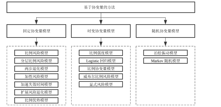
摘要: 作为保障工业过程可靠性和经济性的重要技术,可靠性评估与寿命预测在过去几十年得到了越来越广泛的关注和长足的发展.在实际应用中,由于难以获取复杂、高可靠性设备失效机理的物理模型,数据驱动的可靠性评估与寿命预测方法成为近年来的主流.同时,自动监测技术和传感器技术的快速发展,使得在工程实践中不仅能够获取系统的退化数据,还能得到大量的系统运行环境监测数据,从而使得数据驱动寿命预测中基于协变量的方法得到了广泛应用.本文根据系统运行环境中协变量数据的不同变化规律,将基于协变量方法的可靠性评估模型分为:固定协变量模型、时变协变量模型和随机协变量模型,并分别讨论了各模型的发展现状.最后,讨论了协变量处理中存在的一些挑战及未来的研究方向.Abstract: Reliability assessment and life-time prognostics have been widely concerned and developed fast in the past decades for their importance in industrial processes. Data driven approaches have been popular due to the complexity of failure mechanism about the reliable complex system. With the development of auto-monitoring and sensor technology, it is easy to obtain degradation data and environment information. A large number of methods based on hazard models with covariates have emerged. In this paper we review the state-of-the-art covariate models in the literature. We classify the approaches into three broad types of models, that is, constant models, time-dependent models and stochastic models. We systematically discuss these models and approaches and finally highlight future research challenges.
-
Key words:
- Life-time prognostics /
- data driven /
- reliability /
- covariate
-
乳腺癌是导致女性死亡的主要癌症之一 [1], 它严重影响着女性的身心健康. 早期诊断和早期综合治疗是防止乳腺癌的最有效手段 [2].由于成本低廉, 性价比高、无辐射以及无创伤等原因, 超声成像技术已经成为检测乳腺癌的重要手段.然而, 乳腺超声(Breast ultrasound, BUS)图像往往需要有临床经验的医生来进行判读, 医生判读的准确性又会受到各种内部或外部因素的影响.为了克服这种缺陷, 帮助医生提高诊断的准确率和客观性, 计算机辅助诊断(Computer aided diagnosis, CAD)系统越来越多的被应用于临床实践中 [3-5].
分割是乳腺超声图像CAD系统中重要的一个环节, 通过分割可以定位肿瘤区域的位置, 为后续肿瘤特征提取以及良恶性分类提供必要的信息.由于超声图像具有高噪声、低对比度、边缘模糊不清等特点, 超声图像的分割成为图像处理领域中一个难度较高、亟待解决的问题.近年来, 许多基于不同模型的乳腺肿瘤分割方法已经被提了出来, 例如:区域增长方法(Region growing)[6]、 马尔科夫随机场方法(Markov random field, MRF)[7]、 主动轮廓方法(Active contour)[8]、 神经网络方法(Neural network)[9]、 水平集方法(Level set)[10]等. 国内的学者也提出了许多不同的方法 [11-13].虽然现有的一些分割方法通过结合多种先验知识, 已经取得了较好的效果, 但是这些方法仍然存在一些问题:
1) 乳腺超声图像对比度较低, 而且在图像的脂肪层以及肌肉层存在较多的与肿瘤强度接近的低回声区域, 现有的依赖空间域特征的方法不能有效地将肿瘤与低回声区域区分开来, 特别是当低回声区域与肿瘤区域的边界较为接近时, 现有的方法往往会出现过分割.
2) 现有的乳腺超声图像分割方法都将单帧静态超声图像作为研究对象, 然而单帧静态图像只能反映肿瘤某一侧面的信息.实际临床中, 医生在扫查和诊断中用的是超声视频序列, 这个视频序列与单帧静态图像相比, 可以提供更完整、更全面的肿瘤信息.
为了解决上述问题, 本文提出了一种基于多域先验的协同分割模型来对乳腺超声序列进行分割. 协同分割(Co-segmentation)方法最早由Rother等 [14]提出, 是一种无监督学习的分割方法, 目的是将多幅具有相同或相似目标的图像分割为前景和背景.目前越来越多的人开始对协同分割方法进行研究. 现有的大多数协同分割方法是基于马尔可夫随机场(MRF)的优化问题 [15], 其基本思想是建立起包括图像内部能量项和图像间全局能量项的能量方程, 然后将能量方程转化到MRF问题上进行优化. 这类方法通常是在全局能量项上进行改进, 使全局能量项更合理或者使整个模型的优化更便利. 除了基于MRF的方法外, 还有一些其他的协同分割方法被提出. Joulin等 [16]从聚类的角度出发, 通过将图像内部聚类与全局图像聚类结合起来, 提出了基于聚类的协同分割方法. Kim等 [17]从各向异性热扩散的原理出发, 将协同分割问题视作温度最大化问题来解决. Meng等 [18]通过将多幅图像构建成图, 然后使用最短路径的方法来进行协同分割. 现有的协同分割方法大都是在自然图像上进行分割的, 方法使用的特征也是从自然图像的角度考虑的. 与自然图像相比, 乳腺超声图像有较低的分辨率和对比度, 图像中各个组织之间的边界比较模糊, 图像内部有较多的噪声, 所以已有的协同分割方法在乳腺超声图像中并不适用.
本文提出的多域协同分割模型充分结合了乳腺超声图像的特点.一方面, 通过考虑乳腺超声图像在空间域的强度分布、 位置和姿态信息, 与频率域的边缘信息相结合, 建立起超声图像内部的能量关系; 另一方面, 本文结合了乳腺肿瘤图像的特征来对协同分割框架中的能量项进行了设计, 建立起超声序列之间的全局能量模型.该模型可以有效地利用序列图像特点进行乳腺肿瘤分割.
1. 基于多域先验的协同分割模型
本文提出的多域协同分割模型分割步骤如图 1所示.模型处理的是乳腺超声序列.在使用多域协同分割模型分割之前, 需要对输入序列进行预分割.肿瘤在乳腺超声图像中表现为"颜色相对较暗、团块状"区域.然而, 图像中的肌肉和脂肪组织也有类似的外观.预分割可以给出肿瘤所在区域的位置, 使肿瘤区域成为前景区域, 肌肉、脂肪和其他区域成为背景区域.这是个粗定位的过程, 无法获得肿瘤准确的边界.文献[19]提出了一种基于单帧显著性的乳腺肿瘤检测方法, 文章首先根据医学先验对乳腺肿瘤进行定位, 然后根据乳腺的背景特征以及强度特征构建起解剖学线索和对比度线索, 最终得到乳腺肿瘤的显著性映射结果. 因为文献[20]中的方法具有全自动、 定位准确等特点, 本文用其进行预分割.预分割算法的复杂度为 O$(K^3)$, 其中, K为图像中超像素块的数量.
1.1 分割模型概述
本文提出的多域协同分割模型包括两个部分:内部能量项和全局能量项.为了便于后续表示, 使用$I = \{ {I_k}\} _{k = 1}^M$ 表示含有M帧图像的乳腺超声序列, 使用 ${{x}_{k}} = \{ x_i^k\} _{i = 1}^N$ 表示第${I_k}$帧图像对应的二值标签集合, 其中图像${I_k}$含有的像素个数为N, $x_i^k$表示图像${I_k}$的第i个像素对应的二值标签, $x_i^k$取值为1时其为前景, 取值为0时其为背景.本文的目标是通过多域协同分割模型来实现更优分割, 也就是对标签集合 ${{X}}(\{ {{{x}}_{{k}}}\} _{k = 1}^M)$实现最优分配, 这个问题可以通过最小化式(1)中的能量方程来实现:
$E({{X}}) = {E_{\rm In}} + {E_{\rm Global}} $
(1) 式中, ${E_{\rm In}}$表示单帧图像内部的能量项, 用来约束单帧图像内前景像素与背景像素的关系, ${E_{\rm Global}}$ 表示序列之间的全局能量项, 用来构建序列之间的能量关系.其中${E_{\rm In}}$又分为空域能量项和频域能量项两部分, 所以式(1)可以表示为
$E({{X}}) = \lambda {E_{SC}} + {E_{FC}} + {E_{\rm Global}} $
(2) 式中, ${E_{SC}}$表示空域能量项, 用来对肿瘤的强度、 位置和姿态进行描述. ${E_{FC}}$表示频域能量项, 用来对肿瘤的边缘信息进行描述, ${E_{SC}}$和${E_{FC}}$共同建立起超声图像内部的能量关系. $\lambda$ 是空域能量项的权值, 用于调节空域能量项与频域能量项在模型中所占的比重.以下分别对模型中的各项进行详细说明.
1.2 空域能量项
由于肿瘤区域与低回声区域在强度上具有较大的相似性, 仅使用强度信息很难将之区分, 并容易产生过分割.文献[4]从单帧肿瘤图像的特点出发, 提取了肿瘤姿态、 位置和强度分布等空间域信息来区分肿瘤与正常组织区域, 本文利用文献[4]中的思想, 并将其扩展到序列图像中, 得到了如下的空域能量项表示:
${{E}_{SC}}(X)=\sum\limits_{k=1}^{M}{\left[ \sum\limits_{i}{-\ln (P_{i}^{k}H_{i}^{k})+\sum\limits_{(i, j)\in {{N}_{i}}}{H_{(i, j)}^{k}}} \right]}$
(3) 式中, $P_i^k$是对图像${I_k}$在像素i处的肿瘤姿态与位置描述. $H_i^k$是对图像${I_k}$在像素i处的强度描述, $H_{(i, j)}^k$中像素i处的邻域像素不连续性程度的描述, ${N_i}$表示图像${I_k}$中像素i的邻域集合.
1.2.1 姿态与位置描述
肿瘤的姿态和位置是区分良恶性肿瘤的重要特征, 能不随图像亮度和对比度的变化而变化 [4]. 由于本文使用的所有乳腺超声图像中均只含有一个肿瘤, 所以这里使用2维椭圆高斯方程来表示肿瘤的姿态与位置:
$P_{i}^{k}(x_{i}^{k})=G_{i}^{k}x_{i}^{k}+(1-G_{i}^{k})\bar{x}_{i}^{k}$
(4) $\begin{align} & G_{i}^{k}(i)=\exp \{-[a{{({{i}_{x}}-{{i}_{{{x}_{0}}}})}^{2}}+2b({{i}_{x}}-{{i}_{{{x}_{0}}}})({{i}_{y}}-{{i}_{{{y}_{0}}}})+c{{({{i}_{y}}-{{i}_{{{y}_{0}}}})}^{2}}] \\ & +c{{({{i}_{y}}-{{i}_{{{y}_{0}}}})}^{2}}]\} \\ \end{align}$
(5) 式中, 使用的椭圆由预分割结果中的前景拟合得到, 拟合时, 将前景区域的质心做为椭圆的中心, 将与前景区域具有相同标准二阶中心矩的椭圆的长轴作为椭圆长轴, 将与前景区域具有相同标准二阶中心矩的椭圆的短轴作为椭圆短轴, 将与前景区域具有相同标准二阶中心距的椭圆的长轴与水平轴的夹角作为椭圆的倾角. $({i_{{x_0}}}, {i_{{y_0}}})$和$({i_x}, {i_y})$分别表示图像${I_k}$中椭圆的中心坐标和像素i 处的坐标. $a, b, c$用来控制椭圆的姿态, 参数$a, b, c$由式(6)给出:
$a=\frac{{{\cos }^{2}}\theta }{2\sigma _{x}^{2}}+\frac{{{\sin }^{2}}\theta }{2\sigma _{y}^{2}}, b=-\frac{\sin 2\theta }{4\sigma _{x}^{2}}+\frac{\sin 2\theta }{4\sigma _{y}^{2}}, c=-\frac{{{\sin }^{2}}\theta }{2\sigma _{x}^{2}}+\frac{{{\cos }^{2}}\theta }{2\sigma _{y}^{2}}$
(6) 式中, $\theta$表示椭圆的倾角, ${\sigma _x}$和${\sigma _y}$分别表示1/2长度的椭圆长轴与短轴.椭圆高斯方程能够将分割结果有效地约束在自身的范围内, 排除远离肿瘤区域中与肿瘤区域相似的低回声区域.
1.2.2 强度约束
一些方法在使用强度分布对乳腺超声图像进行分割时, 会先假设图像的强度满足一定的先验分布, 例如: 瑞利(Rayleigh)分布、 伽玛(Gamma)分布或者指数(Exponential)分布等, 由于乳腺超声图像在采集时可能使用不同的设备, 或者使用不同的参数来进行采集, 这些预先定义的强度分布与图像的实际情况会有一定的偏差.因此, 本节在对强度进行定义的时候, 并没有假设图像的强度分布, 而是使用图像的前景与背景直方图来进行表示, 这种表示方法比预先假设强度分布具有更好的鲁棒性. 强度表示的一阶定义如式(7):
$H_i^k(x_i^k) = \Pr (y_i^k|obj)x_i^k + \Pr (y_i^k|bkg)\overline {x}_i^k $
(7) 式中, $y_i^k$表示图像$I_i^k$在像素i处的强度值, $\Pr (y_i^k|obj)$和$\Pr (y_i^k|bkg)$分别表示图像${I_k}$中的像素i属于前景和背景的类条件概率密度, 条件概率密度的值由前景直方图和背景直方图来确定. 图像强度的二阶定义由相邻像素不连续性的程度来定义, 其表示形式如式(8):
$H_{(i, j)}^k = [x_i^k \ne x_j^k]\exp \left(\frac{ -{\left\| {y_i^k -y_j^k} \right\|^2}}{2{\sigma ^2}}\right) $
(8) 式中, $[\phi]$为指示函数, 当 $\phi$为真时, 取值为1; 当$\phi$为假时, 取值为0, $y_i^k$和$y_j^k$分别表示图像${I_k}$ 在像素i和j处的强度值. $H_{(i, j)}^k$表示图像${I_k}$在像素$i $处的不连续性, 当i处比较平滑时, $H_{(i, j)}^k$值相对较小, 当i处不平滑时, $H_{(i, j)}^k$ 值相对越大. $\sigma$ 用来控制不连续性的大小, 实验表明, 当 $\sigma$ 取15时能达到最好效果.
1.3 频域能量项
因为乳腺超声图像在采集时使用的参数会有变动, 其亮度与对比度也会随之变化. 传统的基于空间域的分割方法在检测边缘时, 往往会受到这些变化的影响, 进而不能得到满意的结果. 相位一致性 [20]与零交叉 [21]是两种重要的频率域边缘检测方法, 能够不随图像亮度与对比度的变化而变化, 目前已经被广泛地应用于图像处理领域 [22].本部分将相位一致性与零交叉方法相结合, 构建起了模型的频域能量项:
$\begin{align} &{{E}_{FC}}\left( X \right)=\sum\limits_{k=1}^{M}{\sum\limits_{\left( i, j \right)\in {{N}_{i}}}{ED_{\left( i, j \right)}^{k}=}} \\ &\sum\limits_{k=1}^{M}{\sum\limits_{\left( i, j \right)\in {{N}_{i}}}{\left[ x_{i}^{k}\ne x_{j}^{k} \right]\times ZC_{\left( i, j \right)}^{k}\left( 1-\max \left( PCM_{i}^{k}, PCM_{j}^{k} \right) \right)}} \\ \end{align}$
(9) 式中, $ZC$和$PCM$分别表示零交叉检测与最大能量响应对应的相位一致性值. 本节中相位一致性的计算采用文献[4]中的方法.该方法将图像与一系列不同尺度不同方向的 Log-Gabor滤波器做卷积, 然后进行相位一致性的求解. 滤波器最大响应处对应的尺度和方向能够反映图像局部区域的平滑程度以及方向. 如果一个点在较大的尺度上有较大的响应, 则此点附近的区域较为平滑; 相反, 如果一个点在较小的尺度上有较大的响应, 则此点附近的区域不平滑 [4]. 在方向方面, 如果一个点在方向角$\theta$ 上有较大的响应, 则此点处对应的方向角接近于$\theta$. 因此, 肿瘤边缘的尺度和方向与滤波器的尺度和方向相同时, 滤波器的局部响应最大. 本文中, 选择一个点处Log-Gabor滤波器最大实部${e_{ns, no}}$对应的尺度$(ns)$ 和方向$(no)$作为该点的边缘尺度和方向.
$(s_i^k, n_i^k) = \arg \mathop {\max }\limits_{ns, no} \{ {e_{ns, no}}(i)\}, i \in {I_k} $
(10) 零交叉检测ZC的形式如式(11):
$ZC_{(i, j)}^{k}=\text{ }\frac{1}{2}[1-\text{sgn}({{e}_{(s_{i}^{k}, n_{i}^{k})}}(i))\cdot \text{sgn}({{e}_{(s_{j}^{k}, n_{j}^{k})}}(j))], j\in {{N}_{i}}, i\in {{I}_{k}}$
(11) $ZC_{(i, j)}^k$能够决定点i和j之间是否存在一条边, 如果符号函数${e_{s_i^k, n_i^k}}$与${e_{s_j^k, n_j^k}}$ 相同, 则$ZC_{(i, j)}^k$为0, 说明两点之间不存在边, 如果不相同, 则$ZC_{(i, j)}^k$ 为1, 说明两点之间存在边.
最大能量响应对应的相位一致性值PCM的形式如式(12):
$PCM_{i}^{k}=\cos [{{\varphi }_{(s_{i}^{k}, n_{i}^{k})}}(i)]\text{ }PC_{i}^{k}, i\in {{I}_{k}}$
(12) 式中, $PCM_i^k$能够检测到相位0或$\pi $处的边缘, 由于其构成具有软间隔特性, 所以可以检测到模糊边缘(相位接近0或$\pi $). ${\varphi _{(s_i^k, n_i^k)}}$表示图像${I_k}$在像素i处的相位, $PC_i^k$表示图像${I_k}$在像素i处的相位一致性值. $PC_i^k$的值可以通过文献[23]中的方法得到.
1.4 全局能量项
乳腺超声序列中, 相邻的乳腺超声图像在前景区域具有相似性. 协同分割方法正是从序列图像前景区域的相似性出发构建起全局能量项的, 这种方法通过对多帧图像的前景和背景建模, 得到更准确的前景与背景分布, 进而实现比单帧分割更准确的序列分割.
现在的一些协同分割方法 [24]在构建全局能量项时, 通常是对两幅图像使用强度直方图来进行约束. 由于乳腺超声序列中图像数量多于两幅, 这种只能处理成对图像的方法不能够充分地利用序列信息.因此, 本部分使用了文献[15]中的基于高斯混合模型(Gaussian mixture model, GMM)的方法来定义全局能量项. GMM有以下优点: 1) GMM是一种概率分布模型, 具有较高的准确率; 2) GMM能够详细地描述一个目标不同区域的分布情况.本文中全局能量项的定义如式(13):
${{E}_{\text{Global}}}(X)=\sum\limits_{k=1}^{M}{\sum\limits_{i}{-\ln [\Pr (z_{i}^{k}|{{\theta }_{coobj}})}}x_{i}^{k}+\Pr (z_{i}^{k}|\theta _{bkg}^{k})\overline{x_{i}^{k}}]$
(13) 式中, $\Pr ( \cdot )$为GMM的概率分布, $z_i^k$表示图像${I_k}$在像素i处的特征(强度特征与PCM特征), ${\theta _{coobj}}$ 为图像序列中所有图像前景的GMM参数, $\theta _{bkg}^k$为图像${I_k}$的背景像素的GMM参数, GMM参数的计算过程如下: 首先, 使用K-means算法分别将序列图像的所有前景区域分为$Fc$个类别, 将序列中每帧图像的背景区域分为$Bc$ 个类别, 类别个数即为GMM中高斯模型的个数.然后, 将每个类别中所有像素特征的均值、 协方差矩阵以及本类别中像素占总像素的比例分别作为本类别对应高斯的均值、 协方差矩阵和高斯权重.这样就可以得到前景和背景的GMM参数.实验结果表明, 当$Fc = 3$, $Bc = 5$时有较好的效果.考虑到乳腺超声序列中前景相似的特性, 对${E_{\rm Global}}$ 的最小化能够保证图像序列前景区域的一致性与连续性.
1.5 模型优化
本文的目标是从乳腺超声序列中分割出肿瘤, 这是一个二分割问题. Boykov等提出的交互式图割 [25]为本文模型的优化提供了一种有效的手段. 在图割方法中, 标准的能量方程形式如式(14)所示 [26]:
$E\left( L \right) = \sum\limits_{p \in P} {{D_p}\left( {{L_p}} \right) + \sum\limits_{(p, q) \in N} {{V_{p, q}}\left( {{L_p}, {L_q}} \right)} } $
(14) 式中, $L = \left\{ {{L_p}|p \in P} \right\}$为图像P的标签集合, ${D_p}\left( \cdot \right)$为数据惩罚项, ${V_{p, q}}$为平滑项, N为所有相邻像素对的集合.本文提出的多域协同分割模型中, 式(3)空域能量项中的$P_i^kH_i^k$对应数据惩罚项, $H_{\left( {i, j} \right)}^k$对应平滑项, 式(9)频域能量项对应平滑项, 式(13)全局能量项对应数据惩罚项.这样, 本文提出的模型可以映射到标准能量方程的形式上去. 又因为本文模型满足文献[27]中的图表示形式, 即:
$\begin{align} &H_{\left( i, j \right)}^{k}\left( 0, 0 \right)+H_{\left( i, j \right)}^{k}\left( 1, 1 \right)+ED_{\left( i, j \right)}^{k}\left( 0, 0 \right)+ \\ &ED_{\left( i, j \right)}^{k}\left( 1, 1 \right)\le H_{\left( i, j \right)}^{k}\left( 0, 1 \right)+H_{\left( i, j \right)}^{k}\left( 1, 0 \right)+ED_{\left( i, j \right)}^{k}\left( 0, 1 \right)+ED_{\left( i, j \right)}^{k}\left( 1, 0 \right) \\ \end{align}$
所以本文提出的模型能够使用最大流最小割算法1来进行全局最优化, 模型复杂度为O$\left( {{n^2}m\left| C \right|} \right)$, 其中n为顶点数, m为边数, $\left| C \right|$为最小割的数量.
1.6 算法实现
因为在开始求解模型时, 乳腺超声序列的前景和背景是通过预分割得到的, 预分割结果比较粗糙, 可以通过迭代的方式来对乳腺超声序列进行分割.迭代终止的条件可以为: GMM的参数满足收敛条件, 或者达到最大迭代次数(通常使用5 $\sim$ 10次迭代).完整的分割算法流程如下:
步骤 1. 使用文献[19]中的方法对乳腺图像序列进行预分割;
步骤 2. 使用图割算法对式(1)中的${E_{\rm In}}$进行最小化, 产生初步分割结果;
步骤 3. 初始化GMM的参数${\theta _{coobj}}$, $\theta _{bkg}^k$;
步骤 4. 使用图割算法对式(2)进行最小化;
步骤 5. 根据式(2)的优化结果更新参数$\theta _{coobj}$, $\theta _{bkg}^k$;
步骤 6. 循环执行步骤3和步骤5直到满足收敛条件或者达到最大迭代次数为止.
2. 实验结果
2.1 数据集
为了验证本文提出方法在乳腺超声序列图像上的分割效果, 本文对50组乳腺超声序列进行了分割. 50组序列中包括25组恶性序列和25组良性序列, 每组序列包括5 $\sim$ 12帧图像, 总计400帧图像, 图像的平均大小为600像素 × 480像素. 本文采用的所有乳腺超声图像序列由哈尔滨医科大学附属第二医院超声科提供, 并由超声专家对肿瘤区域进行手工标注, 作为金标准验证分割的效果.本文实验在一台4核2.13 GHz CPU、12 GB内存的计算机上运行, 使用Matlab来进行算法实现, 平均处理一帧图像的时间为10.02 s.
2.2 评价标准
为了对分割效果进行评价, 本文使用了面积和边界两种误差评价标准.其中面积评价标准包括: 真阳性比(True positive ratio, TPR)、假阳性比(False positive ratio, FPR)和总体相似度(Similarity ratio, SIR):
$\text{TPR}=\frac{\left| {{A}_{m}}\cap {{A}_{r}} \right|}{\left| {{A}_{m}} \right|}, \text{FPR}=\frac{\left| {{A}_{m}}\cap {{A}_{r}}-{{A}_{m}} \right|}{\left| {{A}_{m}} \right|}\text{, SIR}=\frac{\left| {{A}_{m}}\cap {{A}_{r}} \right|}{\left| {{A}_{m}}\cup {{A}_{r}} \right|}$
(15) 其中, ${A_m}$表示医生手工标定的肿瘤区域, ${A_r}$为算法分割出的肿瘤区域. TPR指标越高, 则分割结果覆盖手工标定区域的程度越高; FPR指标越低, 则覆盖的错误区域越少; SIR指标越高, 则分割结果与手工标定的区域越接近 [28-29].
豪斯多夫距离(Hausdorff distance, HD)和平均绝对距离(Mean absolute distance, MD)用来评价两个边界的差异程度 [28]. 这里将超声专家标注的边界记为$Q = \left\{ {{q_1}, {q_2}, \cdots , {q_\eta }} \right\}$将分割得到乳腺肿瘤边界记为$P = \{ {p_1}, {p_2}, \cdots, p_j, {p_\alpha }\} $, Q和P对应于同一个肿瘤边界. 对于P上的任意一点${p_j}$, 定义:
$d({p_j}, Q) = \mathop {\min }\limits_w \left\| {{p_j} -{q_w}} \right\|, w = 1, \cdots, \eta $
(16) 其中, $\left\| \cdot \right\|$表示2维欧氏距离, $\alpha $和$\eta $ 分别表示边界P和Q上点的个数. HD和MD的定义如下:
$\text{HD}=\underset{j}{\mathop{\max }}\, d({{p}_{j}}, Q), j=1, \cdots , \alpha $
(17) $\text{MD}=\frac{\sum\limits_{j=1}^{\alpha }{d({{p}_{j}}, Q)}}{\alpha }$
(18) HD表示两个边界的最大不一致程度, MD表示两个轮廓的平均不一致程度. 本文中使用所有肿瘤图像的平均豪斯多夫距离(Average Hausdorff distance, AHD)以及平均绝对误差距离(Average mean absolute distance, AMD)来对分割结果的边界进行评估, AHD与AMD值越大, 分割得到的边界与手工标定的边界差别越大.
2.3 结果
为了全面展示本文提出的模型, 本节首先展示模型的部分中间结果以及模型中参数的变化对最终分割结果的影响. 然后, 将本文提出的模型与三种最新的全自动分割方法 [4, 30-31]进行对比分析, 从模型对与肿瘤相似区域的分割能力, 模型处理低对比度、边界模糊的超声图像的能力以及模型处理单帧分割不容易区分的能力等方面对模型进行评价(由于篇幅有限, 每个序列取3帧图像表示). 实验中, 所有的实验数据均是在相应方法各自的最优参数条件下获得.
图 2显示了本文提出算法的部分中间结果, 图 2(a) 是原始图像序列, 图 2(b) 是原始图像序列的预分割结果, 预分割能够定位肿瘤的位置, 并进行简单分割. 图 2(c) 是乳腺肿瘤序列在空间域中得到的2D高斯椭圆, 用来对肿瘤的姿态与位置进行约束, 从图 2中可以看出, 高斯椭圆能够准确地限制肿瘤区域的位置, 排除背景噪声的干扰.图 2(d) 是乳腺肿瘤序列对应的强度分布序列, 强度图能够有效地利用空间域中的强度信息来表示肿瘤, 图 2(e) 是乳腺肿瘤序列在频率域对应的边缘检测结果, 从图像中可以看出, 最大能量响应处对应的相位一致性值能够明显地表示出肿瘤图像中的边缘信息.图 2(c) 和(d)为空间域中数据项对应的中间结果, 图 2(e) 为频率域的部分中间结果.图 2(f) 是本文提出的多域协同分割模型最后的分割结果.
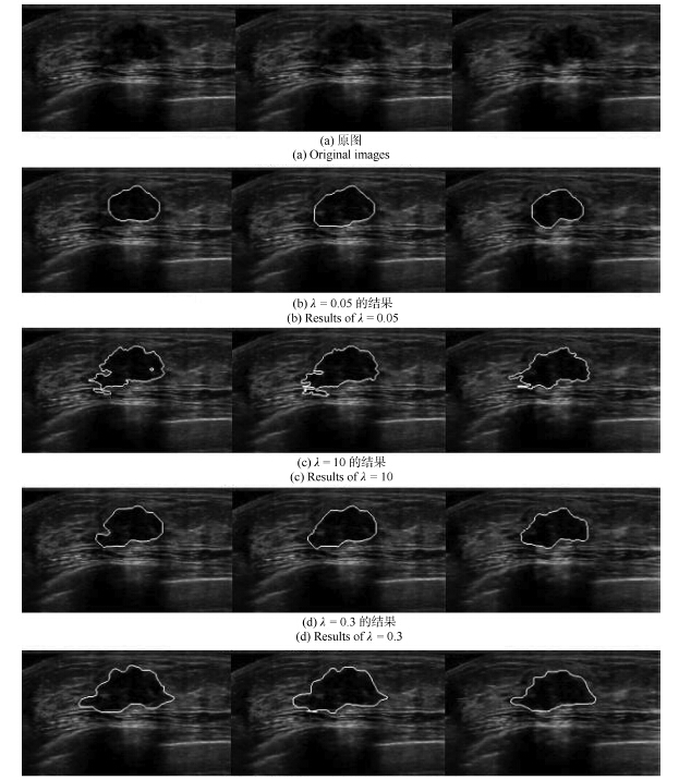
参数$\lambda $用来控制空间域信息和频率域信息对分割结果的影响.当$\lambda $ 较小时, 空域能量项对分割结果的影响较小, 频域能量项对结果的影响较大, 分割结果对边缘信息更为敏感, 容易将疑似边缘区域作为肿瘤边缘. 随着$\lambda $增大, 空域能量项对分割结果的影响逐渐增大.当$\lambda $ 取较大值时, 空域能量项会对分割结果产生较大影响, 分割结果对强度信息更为敏感, 容易将与肿瘤区域近似的组织区域误判断为肿瘤, 产生过分割. 图 3(b) $\sim$ 图 3(d) 分别是采用$\lambda= 0.05$, $\lambda = 10$和$\lambda = 0.3$ 对图 3(a)的序列分割的结果. 采用过小的$\lambda $值($\lambda = 0.05$)时, 模型过多考虑了频率域信息, 而采用过大的$\lambda $值($\lambda = 10$)时, 分割产生了过多细小的区域和曲折的边界曲线, 即过分割. 实验表明, 当$\lambda = 0.3$时, 模型分割出的区域与实际肿瘤区域最相近.
图 4所示的序列中, 肿瘤图像内部含有较多与肿瘤区域相似的正常组织. 图 4(b) $\sim$ (e) 分别是文献[28]提出的基于人工神经网络的模型, 文献[29]提出的基于目标识别的分割模型, 文献[4]提出的基于图分割的模型与本文提出的多域协同分割模型对图 4 (a)所示序列的分割结果. 通过对比图 4 (f)医生标定的肿瘤区域可以看出, 文献[28]中的分割结果中包含较多的正常组织, 文献[4, 29]则正确的区分了肿瘤区域与正常组织. 本文提出的模型最接近医生手工标定的肿瘤区域.
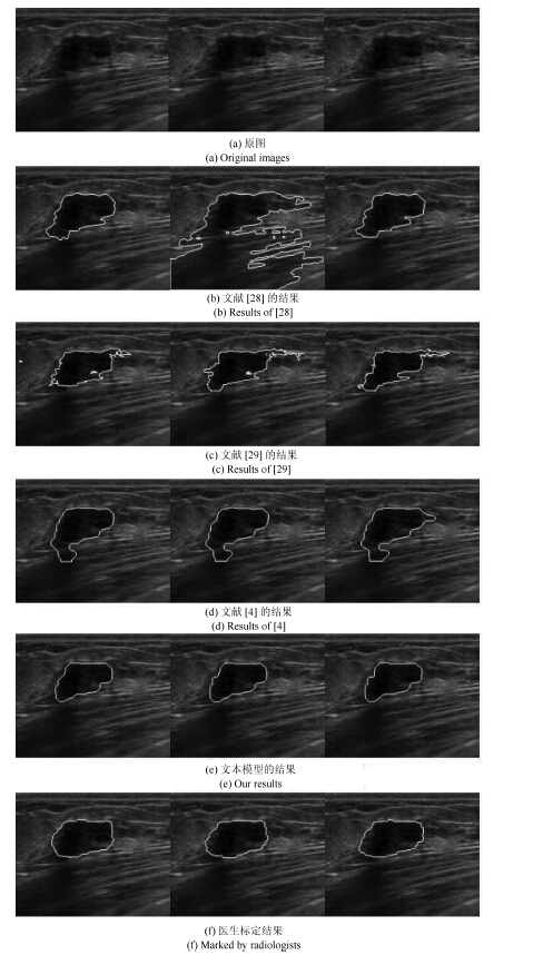 图 4 4 含较多与肿瘤区域相似的正常组织的超声序列分割结果Fig. 4 Segmentation results of normal breast ultrasound sequence similar to tumor regions
图 5展示了4种分割方法在低对比度、边界模糊的乳腺超声序列上的分割结果. 通过对比医生标定的肿瘤区域可以看出, 本文提出的协同分割模型对于低对比度、 边界模糊的超声图像仍可以准确地分割(图 5 (e)), 文献[4]中的方法也得到了相似的结果, 但是其上边缘部分没有完整地收敛到肿瘤的边界. 文献[29]中的方法只能识别部分肿瘤区域, 文献[28]中的方法虽然将肿瘤区域正确识别, 但其结果中包含了较多的正常组织.
 图 5 低对比度、边界模糊的超声序列的分割结果Fig. 5 Segmentation results of breast ultrasound sequence with low contrast and blurry boundaries
图 6和图 7分别是4种分割方法在单帧不容易区分的乳腺超声序列上的分割结果. 观察这些序列中的图像可以看出, 这些序列中部分肿瘤图像对比度较低, 肿瘤内部不均匀, 有部分低回声区域同时也有部分较亮的区域(图 6的2帧图像, 图 7的第2帧图像).在使用单帧分割时, 往往会将肿瘤内部较亮与较暗区域的分界处作为边界, 造成误分割(图 6 (b) $\sim$ (d), 7 (b) $\sim$ (d)). 本文提出的多域协同分割模型能够通过结合序列图像中所有图像的前景信息来进行分割, 利用图像序列的全局信息对分割结果进行纠正, 从而得到正确的结果(图 6 (e)和图 7(e) ).
 图 6 单帧不易分割的超声序列的分割结果Fig. 6 Segmentation results of breast ultrasound sequence hard to segment for single frame
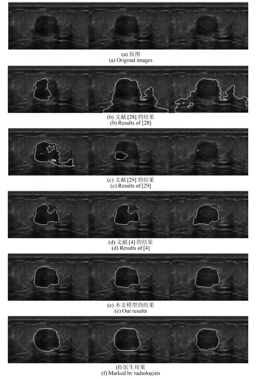 图 7 单帧不易分割的超声序列的分割结果Fig. 7 Segmentation results of breast ultrasound sequence hard to segment for single frame
表 1列出了文献[4, 28-29]中的方法与本文提出的方法在同一数据集上的整体表现. 从结果中可以看出, 文献 [4]中的方法有稍高的TPR (82.61 %)值, 这表明其模型分割得到的肿瘤区域与实际的肿瘤区域有较高的重合部分. 不过, 本文提出的模型有较低的FPR (17.54 %)值和较高的SIR(73.63 %)值, 这表明本文提出的模型能够有效地区分与肿瘤区域相似的正常组织区域.从边界评价标准上来看, 本文的方法也远低于文献[4, 28-29]中的结果, 这表明本文模型得到的分割结果更接近于实际肿瘤边界. 4类方法的受试者工作特征(Receiver operating characteristic curve, ROC)曲线见图 8, 表 2列出了4类方法的AUC (Area under roc curve)值, 从表 2中可以看出, 本文模型的AUC面积最大, 这表明本文模型有最好的分割效果.
表 1 4类方法在所有乳腺超声图像上的整体分割结果Table 1 Segmentation results of four methods on all breast ultrasound images表 2 4 类分割方法的AUC 值Table 2 Results of AUC of four segmentation methods3. 结论
本文提出了一种多域协同分割模型来对乳腺超声图像序列进行分割, 本文的主要贡献有: 1)通过将空域与频域信息结合, 既可以利用空域中肿瘤的姿态、位置与强度特征, 又可以通过频域来得到肿瘤的边缘特征, 使结果的准确性有较大的提升; 2)结合了乳腺肿瘤图像的特征来对现有协同分割框架中的能量项进行设计, 建立起乳腺超声图像序列模型, 有效地利用序列图像特点进行乳腺肿瘤分割.实验结果表明, 本文的方法可以准确地对超声图像序列进行分割.在未来的工作中, 如何更好地利用图像序列前景之间的相似性, 例如肿瘤在形状上的关系, 以及分割多肿瘤图像, 是今后进一步的研究方向.
-
[1] Gorjian N, Ma L, Mittinty M, Yarlagadda P, Sun Y. A review on reliability models with covariates. In: Proceedings of the 4th World Congress on Engineering Asset Management. Athens, Greece: Springer, 2009. 142-157 doi: 10.1007/978-0-85729-320-6_43 [2] 郑建飞, 胡昌华, 司小胜, 张正新, 张鑫.考虑不确定测量和个体差异的非线性随机退化系统剩余寿命估计.自动化学报, 2017, 43 (2):259-270 http://www.aas.net.cn/CN/abstract/abstract19004.shtmlZheng Jian-Fei, Hu Chang-Hua, Si Xiao-Sheng, Zhang Zheng-Xin, Zhang Xin. Remaining useful life estimation for nonlinear stochastic degrading systems with uncertain measurement and unit-to-unit variability. Acta Automatica Sinica, 2017, 43 (2):259-270 http://www.aas.net.cn/CN/abstract/abstract19004.shtml [3] 司小胜, 胡昌华, 周东华.带测量误差的非线性退化过程建模与剩余寿命估计.自动化学报, 2013, 39(5):530-541 http://www.aas.net.cn/CN/abstract/abstract17879.shtmlSi Xiao-Sheng, Hu Chang-Hua, Zhou Dong-Hua. Nonlinear degradation process modeling and remaining useful life estimation subject to measurement error. Acta Automatica Sinica, 2013, 39 (5):530-541 http://www.aas.net.cn/CN/abstract/abstract17879.shtml [4] Liao L X, Kottig F. Review of hybrid prognostics approaches for remaining useful life prediction of engineered systems, and an application to battery life prediction. IEEE Transactions on Reliability, 2014, 63 (1):191-207 doi: 10.1109/TR.2014.2299152 [5] Jardine A K S, Lin D M, Banjevic D. A review on machinery diagnostics and prognostics implementing condition-based maintenance. Mechanical Systems and Signal Processing, 2006, 20 (7):1483-1510 doi: 10.1016/j.ymssp.2005.09.012 [6] Hu C H, Zhou Z J, Zhang J X, Si X S. A survey on life prediction of equipment. Chinese Journal of Aeronautics, 2015, 28 (1):25-33 doi: 10.1016/j.cja.2014.12.020 [7] 周东华, 魏慕恒, 司小胜.工业过程异常检测、寿命预测与维修决策的研究进展.自动化学报, 2013, 39 (6):711-722 http://www.aas.net.cn/CN/abstract/abstract18097.shtmlZhou Dong-Hua, Wei Mu-Heng, Si Xiao-Sheng. A survey on anomaly detection, life prediction and maintenance decision for industrial processes. Acta Automatica Sinica, 2013, 39 (6):711-722 http://www.aas.net.cn/CN/abstract/abstract18097.shtml [8] Cox D R. Regression models and life-tables. Journal of the Royal Statistical Society, 1972, 34 (2):187-220 http://www.jstor.org/stable/2985181 [9] Kumar D, Westberg U. Some reliability models for analyzing the effect of operating conditions. International Journal of Reliability, Quality and Safety Engineering, 1996, 4 (2):133-148 doi: 10.1142/S0218539397000102?queryID=%24%7BresultBean.queryID%7D [10] Anderson J A, Senthilselvan A. A two-step regression model for hazard functions. Applied Statistics, 1982, 31 (1):44-51 doi: 10.2307/2347073 [11] Pijnenburg M. Additive hazards models in repairable systems reliability. Reliability Engineering and System Safety, 1991, 31 (3):369-390 doi: 10.1016/0951-8320(91)90078-L [12] Andersen P K, Vaeth M. Simple parametric and nonparametric models for excess and relative mortality. Biometrics, 1989, 45 (2):523-535 doi: 10.2307/2531494 [13] Shyur H J, Elsayed E A, Luxhoj J T. A general model for accelerated life testing with time-dependent covariates. Naval Research Logistics, 1999, 46 (3):303-321 doi: 10.1002/(ISSN)1520-6750 [14] Ciampi A, Etezadi-Amoli J. A general model for testing the proportional hazards and the accelerated failure time hypotheses in the analysis of censored survival data with covariates. Communications in Statistics-Theory and Methods, 1985, 14 (3):651-667 doi: 10.1080/03610928508828940 [15] McCullagh P. Regression models for ordinal data. Journal of the Royal Statistical Society:Series B (Methodological), 1980, 42 (2):109-142 http://www.jstor.org/stable/2984952 [16] Bennett S. Log-logistic regression models for survival data. Applied Statistics, 1983, 32 (2):165-171 doi: 10.2307/2347295 [17] Liao H T, Zhao W B, Guo H R. Predicting remaining useful life of an individual unit using proportional hazards model and logistic regression model. In: Proceedings of the 2006 Annual Reliability and Maintainability Symposium. Newport Beach, CA, USA: IEEE 2006. 127-132 http://ieeexplore.ieee.org/xpls/icp.jsp?arnumber=1677362 [18] Sun Y, Ma L, Mathew J, Wang W Y, Zhang S. Mechanical systems hazard estimation using condition monitoring. Mechanical Systems and Signal Processing, 2006, 20 (5):1189-1201 doi: 10.1016/j.ymssp.2004.10.009 [19] Jardine A K S, Anderson P M, Mann D S. Application of the Weibull proportional hazards model to aircraft and marine engine failure data. Quality and Reliability Engineering International, 1987, 3 (2):77-82 doi: 10.1002/(ISSN)1099-1638 [20] Aalen O O. Further results on the non-parametric linear regression model in survival analysis. Statistics in Medicine, 1993, 12(17):1569-1588 doi: 10.1002/(ISSN)1097-0258 [21] Gorjian N, Ma L, Mittinty M, Yarlagadda P, Sun Y. The explicit hazard model-Part 1: theoretical development. In: Proceedings of the Prognostics & System Health Management Conference. Macau, China: IEEE, 2010. 167-179 http://ieeexplore.ieee.org/xpls/abs_all.jsp?arnumber=5414565 [22] Sheldon M R. Generalized Poisson shock models. The Annals of Probability, 1981, 9 (5):896-898 doi: 10.1214/aop/1176994318 [23] Jarrow R A, Lando D, Turnbull S M. A Markov model for the term structure of credit risk spreads. Review of Financial Studies, 1997, 10 (2):481-523 doi: 10.1093/rfs/10.2.481 [24] Zhao X J, Fouladirad M, Bérenguer C, Bordes L. Condition-based inspection replacement policies for non-monotone deteriorating systems with environmental covariates. Reliability Engineering and System Safety, 2010, 95 (8):921-934 doi: 10.1016/j.ress.2010.04.005 [25] Banjevic D, Jardine A K S. Calculation of reliability function and remaining useful life for a Markov failure time process. IMA Journal of Management Mathematics, 2006, 17 (2):115-130 doi: 10.1093/imaman/dpi029 [26] Myers L E. Survival functions induced by stochastic covariate processes. Journal of Applied Probability, 1981, 18 (2):523-529 doi: 10.2307/3213300 [27] Berman S M, Frydman H. Parametric estimation of hazard functions with stochastic covariate processes. Sankhyā:The Indian Journal of Statistics, 1999, 61 (2):174-188 http://www.ams.org/mathscinet-getitem?mr=1714869 [28] Yu J C, Liu Y Y, Cai J W, Sandler D P, Zhou H B. Outcome-dependent sampling design and inference for Cox's proportional hazards Model. Journal of Statistical Planning and Inference, 2016, 178 (5):24-36 http://www2.cscc.unc.edu/impact7/node/771 [29] Lin H Z, He Y, Huang J. A global partial likelihood estimation in the additive Cox proportional hazards model. Journal of Statistical Planning and Inference, 2016, 169 (9):71-87 https://www.researchgate.net/publication/282528853_A_global_partial_likelihood_estimation_in_the_additive_Cox_proportional_hazards_model [30] Cao Y X, Yu J C, Liu Y Y. Optimal generalized case-cohort analysis with Cox's proportional hazards model. Acta Mathematicae Applicatae Sinica, 2015, 31 (3):841-854 doi: 10.1007/s10255-015-0555-4 [31] Luo J, Su Z. A note on variance estimation in the Cox proportional hazards model. Journal of Applied Statistics, 2013, 40 (5):1132-1139 doi: 10.1080/02664763.2013.780161 [32] Cox D R. Partial likelihood. Biometrika, 1975, 62 (2):269-276 doi: 10.1093/biomet/62.2.269 [33] Kalbfleisch J D, Prentice R L. Marginal likelihoods based on Cox's regression and life model. Biometrika, 1973, 60 (2):267-278 doi: 10.1093/biomet/60.2.267 [34] Makis V, Jardine A K S. Optimal replacement policy for a general model with imperfect repair. Journal of the Operational Research Society, 1992, 43 (2):111-120 doi: 10.1057/jors.1992.17 [35] Banjevic D, Jardine A K S, Makis V, Ennis M. A Control-Limit Policy And Software For Condition-Based Maintenance Optimization. INFOR:Information Systems and Operational Research, 2001, 39(1):32-50 doi: 10.1080/03155986.2001.11732424 [36] Jardine A K S, Banjevic D, Makis V. Optimal replacement policy and the structure of software for condition-based maintenance. Journal of Quality in Maintenance Engineering, 1997, 3 (2):109-119 doi: 10.1108/13552519710167728 [37] Jardine A K S, Joseph T, Banjevic D. Optimizing condition-based maintenance decisions for equipment subject to vibration monitoring. Journal of Quality in Maintenance Engineering, 1999, 5 (3):192-202 doi: 10.1108/13552519910282647 [38] Vlok P J, Wnek M, Zygmunt M. Utilising statistical residual life estimates of bearings to quantify the influence of preventive maintenance actions. Mechanical Systems and Signal Processing, 2004, 18 (4):833-847 doi: 10.1016/j.ymssp.2003.09.003 [39] Kay R. Proportional hazard regression models and the analysis of censored survival data. Applied Statistics, 1977, 26 (3):227-237 doi: 10.2307/2346962 [40] Kumar D. Proportional hazards modelling of repairable systems. Quality and Reliability Engineering International, 1995, 11 (5):361-369 doi: 10.1002/(ISSN)1099-1638 [41] Hanson T, Jara A, Zhao L P. A Bayesian semiparametric temporally-stratified proportional hazards model with spatial frailties. Bayesian Analysis, 2012, 7 (1):147-188 doi: 10.1214/12-BA705 [42] Fibrinogen Studies Collaboration. Measures to assess the prognostic ability of the stratified Cox proportional hazards model. Statistics in Medicine, 2009, 28 (3):389-411 doi: 10.1002/sim.v28:3 [43] Mau J. On a graphical method for the detection of time-dependent effects of covariates in survival data. Applied Statistics, 1986, 35 (3):245-255 doi: 10.2307/2348023 [44] Aalen O O. A linear regression model for the analysis of life times. Statistics in Medicine, 1989, 8 (8):907-925 doi: 10.1002/(ISSN)1097-0258 [45] Newby M. Why no additive hazards models? IEEE Transactions on Reliability, 1994, 43 (3):484-488 doi: 10.1109/24.326450 [46] Newby M. A critical look at some point-process models for repairable systems. IMA Journal of Management Mathematics, 1992, 4 (4):375-394 doi: 10.1093/imaman/4.4.375 [47] Álvarez E E, Ferrario J. Robust estimation in the additive hazards model. Communications in Statistics:Theory & Methods, 2016, 45 (4):906-921 doi: 10.1080/03610926.2013.853790 [48] Wightman D, Bendell T. Comparison of proportional hazards modeling, additive hazards modeling and proportional intensity modeling when applied to repairable system reliability. International Journal of Reliability, Quality and Safety Engineering, 1995, 2 (1):23-34 doi: 10.1142/S0218539395000046 [49] Badía F G, Berrade M D, Campos C A. Aging properties of the additive and proportional hazard mixing models. Reliability Engineering & System Safety, 2002, 78 (2):165-172 https://www.sciencedirect.com/science/article/pii/S0951832002001564 [50] Cox D R, Oakes D. Analysis of Survival Data. New York:Chapman and Hall, 1984. 32-37 [51] Lin Z, Fei H. A nonparametric approach to progressive stress accelerated life testing. IEEE Transactions on Reliability, 1991, 40 (2):173-176 doi: 10.1109/24.87123 [52] Mettas A. Modeling and analysis for multiple stress-type accelerated life data. In: Proceedings of the 2000 Annual Reliability and Maintainability Symposium. Los Angeles, CA, USA: IEEE 2000. 138-143 http://ieeexplore.ieee.org/xpls/abs_all.jsp?arnumber=816297 [53] Gosho M, Maruo K, Sato Y. Effect of covariate omission in Weibull accelerated failure time model:a caution. Biometrical Journal, 2014, 56 (6):991-1000 doi: 10.1002/bimj.201300006 [54] Newby M. Accelerated failure time models for reliability data analysis. Reliability Engineering & System Safety, 1988, 20 (3):187-197 https://www.researchgate.net/publication/222366290_Accelerated_failure_time_models_for_reliability_data_analysis_Reliability_Engineering_System_Safety_203_187-197 [55] Galanova N S, Lemeshko B Y, Chimitova E V. Using nonparametric goodness-of-fit tests to validate accelerated failure time models. Optoelectronics, Instrumentation and Data Processing, 2012, 48 (6):580-592 doi: 10.3103/S8756699012060064 [56] Wang H, Dai H, Fu B. Accelerated failure time models for censored survival data under referral bias. Biostatistics, 2013, 14 (2):313-326 doi: 10.1093/biostatistics/kxs041 [57] Yang M G, Chen L H, Dong G H. Semiparametric Bayesian accelerated failure time model with interval-censored data. Journal of Statistical Computation and Simulation, 2015, 85 (10):2049-2058 doi: 10.1080/00949655.2014.915400 [58] Wang S Y, Hu T, Xiang L M, Cui H J. Generalized M-estimation for the accelerated failure time model. Statistics, 2016, 50 (1):114-138 doi: 10.1080/02331888.2015.1032970 [59] Etezadi-Amoli J, Ciampi A. Extended hazard regression for censored survival data with covariates:a spline approximation for the baseline hazard function. Biometrics, 1987, 43 (1):181-192 doi: 10.2307/2531958 [60] Louzada-Neto F. Extended hazard regression model for reliability and survival analysis. Lifetime Data Analysis, 1997, 3 (4):367-381 doi: 10.1023/A:1009606229786 [61] Tseng Y K, Su Y R, Mao M, Wang J L. An extended hazard model with longitudinal covariates. Biometrika, 2015, 102 (1):135-150 doi: 10.1093/biomet/asu058 [62] Tseng Y K, Hsu K N, Yang Y F. A semiparametric extended hazard regression model with time-dependent covariates. Journal of Nonparametric Statistics, 2014, 26 (1):115-128 doi: 10.1080/10485252.2013.836521 [63] Shyur H J, Keng H, Ia-Ka I, Huang C L. Using extended hazard regression model to assess the probability of aviation event. Applied Mathematics and Computation, 2012, 218 (21):10647-10655 doi: 10.1016/j.amc.2012.04.029 [64] Bennett S. Analysis of survival data by the proportional odds model. Statistics in Medicine, 1983, 2 (2):273-277 doi: 10.1002/(ISSN)1097-0258 [65] Zahid F M, Ramzan S, Heumann C. Regularized proportional odds models. Journal of Statistical Computation and Simulation, 2015, 85 (2):251-168 doi: 10.1080/00949655.2013.814133 [66] Sinha S, Ma Y Y. Analysis of proportional odds models with censoring and errors-in-covariates. Journal of the American Statistical Association, 2016, 111 (515):1301-1312 doi: 10.1080/01621459.2015.1093943 [67] Zahid F M, Tutz G. Proportional odds models with high-dimensional data structure. International Statistical Review, 2013, 81 (3):388-406 doi: 10.1111/insr.v81.3 [68] Landers T L, Soroudi H E. Robustness of a semi-parametric proportional intensity model. IEEE Transactions on Reliability, 1991, 40 (2):161-164 doi: 10.1109/24.87120 [69] Lugtigheid D, Jardine Andrew K S, Jiang X Y. Optimizing the performance of a repairable system under a maintenance and repair contract. Quality and Reliability Engineering International, 2007, 23 (8):943-960 doi: 10.1002/(ISSN)1099-1638 [70] Kumar D, Westberg U. Proportional hazards modeling of time-dependent covariates using linear regression:a case study. IEEE Transactions on Reliability, 1996, 45 (3):386-392 doi: 10.1109/24.536990 [71] Jiang S T, Landers T L, Rhoads T R. Proportional intensity models robustness with overhaul intervals. Quality and Reliability Engineering International, 2006, 22 (3):251-263 doi: 10.1002/(ISSN)1099-1638 [72] Prentice R L, Williams B J, Peterson A V. On the regression analysis of multivariate failure time data. Biometrika, 1981, 68 (2):373-379 doi: 10.1093/biomet/68.2.373 [73] Yuan F Q, Kumar U. Proportional Intensity Model considering imperfect repair for repairable systems. International Journal of Performability Engineering, 2013, 9(2):163-174 http://paris.utdallas.edu/IJPE/Vol09/Issue02/pp.163-174%20Paper%204%20IJPE%20407.12%20Fuqing.pdf [74] Percy D F, Kobbacy K A H, Ascher H E. Using proportional-intensities models to schedule preventive-maintenance intervals. IMA Journal of Management Mathematics, 1998, 9 (3):289-302 doi: 10.1093/imaman/9.3.289 [75] Alkali B. Evaluation of generalised proportional intensities models with application to the maintenance of gas turbines. Quality and Reliability Engineering International, 2012, 28 (6):577-584 https://www.deepdyve.com/lp/wiley/evaluation-of-generalised-proportional-intensities-models-with-fZ2VbgUKzF [76] Syamsundar A, Achutha Naikan V N. Imperfect repair proportional intensity models for maintained systems. IEEE Transactions on Reliability, 2011, 60 (4):782-787 doi: 10.1109/TR.2011.2161110 [77] Wu J B. Modified restricted Liu estimator in logistic regression model. Computational Statistics, 2016, 31 (4):1557-1567 doi: 10.1007/s00180-015-0609-3 [78] Li C S. A test for the linearity of the nonparametric part of a semiparametric logistic regression model. Journal of Applied Statistics, 2016, 43 (3):461-475 doi: 10.1080/02664763.2015.1070803 [79] Sun Y, Ma L. Notes on "mechanical systems hazard estimation using condition monitoring"-Response to the letter to the editor by Daming Lin and Murray Wiseman. Mechanical Systems and Signal Processing, 2007, 21 (7):2950-2955 doi: 10.1016/j.ymssp.2007.06.004 [80] Cai G G, Chen X F, Li B, Chen B J, He Z J. Operation reliability assessment for cutting tools by applying a proportional covariate model to condition monitoring information. Sensors, 2012, 12 (10):12964-12987 http://www.mdpi.com/1424-8220/12/10/12988 [81] Pettitt A N, Daud I B. Investigating time dependence in Cox's proportional hazards model. Applied Statistics, 1990, 39 (3):313-329 doi: 10.2307/2347382 [82] Jardine A K S. Component and system replacement decisions. Image Sequence Processing and Dynamic Scene Analysis. Berlin:Springer-Verlag, 1983. 647-654 [83] Jardine A K S, Ralston P, Reid N, Stafford J. Proportional hazards analysis of diesel engine failure data. Quality and Reliability Engineering International, 1989, 5 (3):207-216 doi: 10.1002/(ISSN)1099-1638 [84] Jóźwiak I J. An introduction to the studies of reliability of systems using the Weibull proportional hazards model. Microelectronics Reliability, 1997, 37 (6):915-918 doi: 10.1016/S0026-2714(96)00285-5 [85] Jardine A K S, Anders M. Use of concomitant variables for reliability estimation. Maintenance Management International, 1985, 5 (4):135-140 https://www.researchgate.net/publication/291839844_USE_OF_CONCOMITANT_VARIABLES_FOR_RELIABILITY_ESTIMATION [86] Newby M. Perspective on Weibull proportional-hazards models. IEEE Transactions on Reliability, 1994, 43 (2):217-223 doi: 10.1109/24.294993 [87] Sha N J, Pan R. Bayesian analysis for step-stress accelerated life testing using Weibull proportional hazard model. Statistical Papers, 2014, 55 (3):715-726 doi: 10.1007/s00362-013-0521-2 [88] Zhang Q, Hua C, Xua G H. A mixture Weibull proportional hazard model for mechanical system failure prediction utilising lifetime and monitoring data. Mechanical Systems and Signal Processing, 2014, 43 (1-2):103-112 doi: 10.1016/j.ymssp.2013.10.013 [89] Gorjian N, Mittinty M, Ma L, Yarlagadda P, Sun Y. The explicit hazard model-Part 2: applications. In: Proceedings of the 2010 Prognostics and Health Management Conference. Macau, China: IEEE, 2010. 189-202 http://ieeexplore.ieee.org/xpls/abs_all.jsp?arnumber=5413493 [90] Cha J H, Mi J. Study of a stochastic failure model in a random environment. Journal of Applied Probability, 2007, 44 (1):151-163 doi: 10.1239/jap/1175267169 [91] Cha J H, Lee E Y. An extended stochastic failure model for a system subject to random shocks. Operations Research Letters, 2010, 38 (5):468-473 doi: 10.1016/j.orl.2010.06.004 [92] Cha J H, Mi J. On a stochastic survival model for a system under randomly variable environment. Methodology and Computing in Applied Probability, 2011, 13 (3):549-561 doi: 10.1007/s11009-010-9171-1 [93] Junca M, Sanchez Silva M. Optimal maintenance policy for a compound Poisson shock model. IEEE Transactions on Reliability, 2013, 62 (1):66-72 doi: 10.1109/TR.2013.2241193 [94] Jiang H Y. Parameter estimation of the Poisson shock model using masked data. International Journal of Pure and Applied Mathematics, 2011, 71 (4):559-569 https://www.researchgate.net/publication/264993406_Parameter_estimation_of_the_Poisson_shock_model_using_masked_data [95] Pandey A, Mitra M. Poisson shock models leading to new classes of non-monotonic aging life distributions. Microelectronics and Reliability, 2011, 51 (12):2412-2415 doi: 10.1016/j.microrel.2011.04.001 [96] Ghasemi A, Yacout S, Salah-Ouali M. Evaluating the reliability function and the mean residual life for equipment with unobservable states. IEEE Transactions on Reliability, 2010, 59 (1):45-54 doi: 10.1109/TR.2009.2034947 [97] Çinlar E. Markov additive processes. I. Zeitschrift für Wahrscheinlichkeitstheorie und Verwandte Gebiete, 1972, 24 (2):85-93 http://en.cnki.com.cn/Article_en/CJFDTOTAL-WHDY404.003.htm 期刊类型引用(2)
1. 张华扬,王铁超. 基于观测器的切换模糊系统的事件触发控制. 模糊系统与数学. 2019(01): 92-101 .  百度学术
百度学术2. 朱芳来,蔡明,郭胜辉. 离散切换系统观测器存在性讨论及降维观测器设计. 自动化学报. 2017(12): 2091-2099 . 本站查看其他类型引用(4)
-


 下载:
下载:


 下载:
下载:
计量
- 文章访问数: 3143
- HTML全文浏览量: 756
- PDF下载量: 1880
- 被引次数: 6
