

-
摘要: 维数约简作为机器学习的经典问题之一,主要用于处理维数灾问题、帮助加速算法的计算效率和提高可解释性以及数据可视化.传统的维数约简算法如主成分分析(Principal component analysis,PCA)和线性判别分析等只能处理无标签数据或者分类数据.然而,当预测变量为一元或多元连续型实值变量时,这些处理无标签数据或分类数据的维数约简方法则不能形成有效的预测性能.近20年来,有一系列工作从多个角度对这一问题展开了研究,并取得了系统性的研究成果.在此背景下,本文将综述这些面向回归问题的降维算法,即实值多变量维数约简.本文将介绍与实值多变量维数约简密切相关的基本概念、算法、理论,并探讨一些潜在的研究方向.Abstract: As one of the classical problems in machine learning, dimension reduction is used for dealing with the curse of dimensionality, speeding up computational efficiency of the algorithm, and improving interpretability as well as visualizing high-dimensional data. Traditional dimension reduction algorithms such as principal component analysis (PCA) and linear discriminant analysis are mainly suitable for unlabeled data or classification data. When the response variables are univariate or multivariate continuous real-valued ones, however, such dimension reduction methods cannot guarantee the effective predictive performance of the reduced subspace. In the recent two decades, researchers have been devoted to studying this issue with different viewpoints, attaining many promising and systemic achievements. Under this background, we will survey the developments of real-valued multivariate dimension reduction in detail. We will also introduce its basic concepts, algorithms and theories, and discuss some potential research directions deserving investigating.
-
集束型设备已被广泛地应用于半导体制造的晶圆加工中[1-2].由于集束型设备加工晶圆时存在多重入流、驻留及资源约束等现象[3],使得集束型设备的调度变得非常复杂.近年来,为了提高设备的产能,集束型设备的结构随着不断改进也出现很多不同的变化,其中一些学者另辟蹊径,希望通过合理地设置缓冲模块来提高设备的产能[4].而对于增加缓冲模块的新型结构的集束型设备来说,现有的调度方法定然不能满足其生产要求,这就需要新的调度方法来支持其调度.
集束型设备一般由多个晶圆加工模块(Processing module,PM)、一个晶圆搬运模块(Transport module,TM)和负责晶圆输入输出的卡匣模块(Cassette modules,CM) 组成.作为晶圆加工特有的工艺要求,驻留约束限制了晶圆在加工模块完成加工后所能停留的时间上限(Upper bound) ,即当晶圆在加工完成后,必须在规定时间范围内离开加工模块,否则残余气体或不适宜温度会导致晶圆出现质量问题,甚至不良品.驻留现象广泛存在于半导体制造过程中[5].针对一般的驻留约束问题,大部分研究都是通过调整晶圆的加工开始时间来满足晶圆的驻留约束[6],一些学者通过设置缓冲模块的方法,使晶圆在加工完成后能够尽早离开加工模块,释放资源,提前下一个晶圆的加工开始时间.
目前,对于一般的集束型设备的周期调度研究已经比较成熟. Perkinson等[7] 与Venkatesh等[8]在不考虑驻留约束的情况下,分别采用推策略和交换策略来获得单臂与双臂集束型设备的最优的基本周期(Fundamental period,FP). Lim等[9] 为了有效提高整体调度周期,考虑晶圆搬运延迟,并提出了一个基于时间表技术的有效实时调度算法.
然而,前面的文献没有考虑驻留约束对集束型设备的调度影响.目前已有相关文献对带驻留约束的集束型设备调度问题进行了研究,Wu等[10]为带驻留约束的集束型设备建立了Petri-网模型,提出了一个封闭式调度算法来获得最优周期的调度.Rostami等[11]运用线性规划和启发式算法来调度带驻留约束的单集束型设备.Zhou等[12]提出了基于侦误的调度启发式算法用于解决带驻留约束的集束型设备调度问题.Rostami等[13]对集束型设备带有加工模块和搬运模块的双驻留约束模型提出了一种调度算法,得到了问题的近优解.
上述文献虽然考虑了驻留约束,却没有考虑缓冲模块对设备产能的影响.对于集束型设备的缓冲模块的研究目前正在起步,Ding等[14]在集束型设备群的研究中,对各个集束型之间的缓冲连接进行了研究.Dawande等[15]比较了制造单元里带输出缓冲和无缓冲的模型,证明带有输出缓冲的制造单元比双爪不带缓冲的制造单元的生产率提高了20%.Drobouchevitch等[16]表明在制造单元的每个机器已存在输出缓冲的基础上增加一个输入缓冲不会提高设备的产能.
上述文献表明,目前对同时带驻留约束和缓冲模块的集束型设备调度问题尚无人研究.本文旨在上述文献的研究基础上,对带驻留约束的集束型设备进行了研究,通过在加工模块之间设置缓冲模块的方法,提高系统产能.该调度问题主要是确定优化的搬运顺序和搬运时间点以获得最小的周期调度.首先,对调度问题在不同搬运模式下建立了相应数学模型;再提出两种不同的调度算法;最后,评价算法的同时,分析缓冲对系统产能的影响.
1. 问题描述
集束型设备里,晶圆由卡匣模块进入,按顺序到每个加工模块加工,完成所有加工后回到卡匣模块.本文的研究对象为加工模块之间带有缓冲模块的单臂集束型设备,如图 1所示.
为有效地描述带缓冲的集束型晶圆制造设备的调度问题,做如下的基本定义与假设:1) 加工模块,搬运模块和缓冲模块在同一时间均只能处理一个晶圆.2) 加工模块上存在驻留约束现象.3) 搬运模块搬运晶圆的时间和装卸时间是确定的.4) 每个晶圆的加工工艺流程都相同.5) 若晶圆进入缓冲模块,缓冲模块被视作虚拟的加工模块,其加工时间为零,且不存在驻留约束;否则,晶圆跳过缓冲模块直接到下一个加工模块进行加工.6) 晶圆在卡匣模块供应充足,晶圆完成最后一道加工工序后直接被搬运到卡匣模块.
为了清晰地表述调度问题,现定义如下符号与变量:
$m$ : 集束型设备加工模块的数量.
$p_i$ : 晶圆 $j$ 在加工模块 $i$ 上的加工时间.
$\delta_i$ : 搬运模块把晶圆从 $M_i$ 搬运到 $M_{i+1}$ 的时间,包括装载和卸载晶圆的时间 $\delta_i=\delta$ .
$\theta_{ij}$ : 搬运模块从 $M_i$ 到 $M_j$ 的空移动的时间 $\theta_{ij}=\min(|i-j|,2m-|i-j|)\cdot\theta$ .
$λ_k$ : 表示晶圆 $j$ 是否经过模块 $M_k$ ,如果是,那么 $λ_k=1$ ;否则, $λ_k=0$ .
$\varphi(i)$ : 表示搬运模块从第 $\varphi(i)$ 模块搬运到 $(\varphi(i)+2-λ_{\varphi(i)+1})$ 模块.
$s_j$ : 搬运模块的搬运模式.
$T$ : 生产每个晶圆的周期时间.
定义 1. 一个单元搬运模式(One-unit TM move style)是指一个晶圆进入加工模块到下一个晶圆开始进入加工模块之间的搬运模块的所有搬运动作.可以通过如下形式来表示: $s=[\varphi(0) ,\varphi(1) ,\varphi(2) ,\cdots,\varphi(m)]$ ,其中 $s$ 是由 $\{0,1,2,\cdots,m\}$ 的排列组成.
由于搬运模式的重复性,假设 $\varphi(0)=0$ ,不失一般性, $\varphi[i\pm(\sum_{k=0}^{2m-1}\lambda_k+1)]=\varphi(i)$ . 两个加工模块的单集束型设备的搬运模式包括如下: $s_1=[0,1,3]$ , $s_2=[0,3,1]$ , $s_3=[0,1,2,3]$ , $s_4=[0,1,3,2]$ , $s_5=[0,2,1,3]$ , $s_6=[0,2,3,1]$ , $s_7=[0,3,1,2]$ , $s_8=[0,3,2,1]$ .
定义 2. 给定一个搬运模式 $s$ ,其中 $\varphi(k)=i$ ,那么 $\varphi(k)$ 的反函数为 $\varphi^-(k)$ , $0\leq\varphi^-(k)\leq m$ , $k=0,1,\cdots,m$ , $\varphi^-(\varphi(i))=i$ ,且 $\varphi(\varphi^-(k))=k$ .
从定义可知,对给定的搬运模式来说,如果搬运模块从 $M_k$ 卸载晶圆,该搬运动作处于单元搬运模式的 $\varphi^-(k)$ th位置,那么当存在 $\varphi^-(k)>\varphi^-(k-2+λ_{k-1})$ 时,从 $M_k$ 装载和卸载的同一片晶圆的搬运动作处于同一个单元搬运模式内;当存在 $\varphi^-(k)<\varphi^-(k-2+λ_{k-1})$ 时,从 $M_k$ 装载和卸载的同一片晶圆的搬运动作却分别处于两个先后的单元搬运模式内.所以 $u_k$ 被定义如下:
\begin{align}u_k=\left\{\begin{array}{c}1,\quad \varphi^-(k)<\varphi^-(k-2+λ_{k-1})\\0,\quad \varphi^-(k)>\varphi^-(k-2+λ_{k-1})\end{array} \right. \end{align}
(1) 任何单元搬运模式内都存在一些不可避免的搬运动作,如晶圆卸载和装载、晶圆的搬运等,用 $IC(s)$ 来表示给定单元搬运模式 $s$ 中必然存在的搬运动作,其表达式如下:
$IC(s)=\sum\limits_{i=0}^{2m-1}{(}{{\delta }_{\varphi (i)}}+{{\theta }_{\varphi (i)}}+2-{{\lambda }_{\varphi (i)+1}},\varphi (i+2-{{\lambda }_{i+1}}))\text{ }$
(2) 在单元搬运模式 $s$ 下,一片晶圆从装载至模块 $M_k$ 到加工完后被卸载这段时间内,搬运模块所耗费的所有的繁忙时间用 $z_k(s)$ 表示:
${{z}_{k}}(s)={{\theta }_{k,{{\tau }_{k}}(s)}}+\sum\limits_{i}^{{{b}_{k}}}{(}{{\delta }_{\varphi (i)}}+{{\theta }_{\varphi (i)}}+2-{{\lambda }_{\varphi (i)+1}},\varphi (i+2-{{\lambda }_{i+1}}))$
(3) 其中, $\tau_k(s)$ 为搬运动作 $k-1$ 的下一搬运动作,即 $\tau_k(s)=\varphi[\varphi^-(k-2+λ_{k-1})+1]$ ,而 $i$ 的初始值为: $\varphi^-(k-2+λ_{k-1})+1$ ,且 $b_k=\varphi^-(k)-1+u_k(\sum_{j=0}^{2m}λ_j+1) $ .
若存在常数 $T$ 使得集束型设备生产状态经 $T$ 时间回到相同的状态,则该时间 $T$ 被称作周期时间.
令 $w_{kj}$ 是指搬运模块在 $M_k$ 等待搬运晶圆 $j$ 的时间.由于周期生产的性质,假设 $\sigma(j\pm n)=\sigma(j)$ , $w_{k,\sigma(j\pm n)}=w_{k,\sigma(j)}$ ,从假设5) 和6) 可知,当 $k$ 是偶数时, $w_{kj}=0$ .
若 $T(s)$ 是相应的搬运模式 $s$ 的周期时间,则目标函数 $T(s)$ 就有:
\begin{align}T(s)=\min\left(IC(s)+\sum_{j=1}^n\sum_{k=0}^mw_{kj}\right) \end{align}
(4) 由加工时间需求的约束与假设1) 可知,晶圆在 $M_k$ 上加工需满足如下约束:
$\sum\limits_{i}^{{{\varphi }^{-}}(k)}{{{w}_{\varphi (i)}}}\ge \max ({{p}_{k}}-{{z}_{k}},0),{{u}_{k}}=0$
(5) $\sum\limits_{i=1}^{\Sigma {{\lambda }_{l}}}{+}\sum\limits_{i}^{{{\varphi }^{-}}(k)}{{{w}_{\varphi (i)}}}\ge \max ({{p}_{k}}-{{z}_{k}},0),{{u}_{k}}=1$
(6) 其中,式(5) 和式(6) 中 $i$ 的初始值为: $i=\varphi^-(k-2+λ_{k-1})+2-λ_{\varphi^-(k-2+λ_{k-1})+1}$ .
由假设2) 的驻留约束有:
\begin{align}z_k-p_k\leq a_k \end{align}
(7) 搬运模块的等待时需满足非负:
\begin{align}w_k\geq 0 \end{align}
(8) 所以,对于给定的搬运模式 $s$ ,要优化目标函数(4) ,服从约束(5) $\sim$ (8) .其中的 $IC(s)$ 与决策变量 $w_{kj}$ 相互独立.
本文是在搬运模式下建立相应的数学模型,在前面数学建模里,该模型的复杂度为 ${\rm O}(m× n)$ ,是多项式内可以求解. 而搬运模式的规模为 ${\rm O}((m+2) m!)$ ,那么整个问题解空间的规模为 ${\rm O}(n(m^2+2m)m!)$ .所以对于问题的求解分为两个阶段:加工等待时间优化和晶圆搬运顺序优化.然后分别构建全局搜索算法和分枝搜索算法对问题进行求解.
2. 全局搜索算法
在集束型设备中,为了方便构建算法,提出以下引理:
引理 1. 生产单晶圆类型的集束型设备,使用超过两个单元搬运模式一般都不是最优的搬运策略.
证明. 假设 $T_i^h$ 是在 $s_i$ 搬运模式下的周期时间, $T_i^h$ 表示在 $s_i$ 搬运模式下的周期时间,且有 $T_i^h=T_j^h$ .那么 $2T_i^h$ 就是在 $s_i$ 下生产两个晶圆的时间,而 $2T_j^h$ 为在 $s_j$ 下生产两个晶圆的时间.如果有 $T_i^h\geq T_j^h$ ,则 $2T_i^h\geq T_i^h+T_j^h\geq 2T_j^h$ ;否则,如果 $T_i^h\leq T_j^h$ ,则有 $2T_i^h\leq T_i^h+T_j^h\leq 2T_j^h$ .可知 $T_i^h+T_j^h$ 不可能小于 $\min(2T_i^h,2T_j^h)$ 的,即两种搬运模式的组合一般不是最优策略.对于超过两个周期的情况证法相似.
定理 1.生产单晶圆类型的集束型设备,最优的搬运策略必定是单一的搬运模式.
证明. 假设 $\Omega$ 为所有的搬运策略集合, $\Omega$ 由 $k$ 个集合即 $\{\Omega_1,\Omega_2,\cdots,\Omega_k\}$ 组成,其中 $\Omega_k$ 表示 $k$ 种不同搬运模式组成的搬运策略集合,那么必有最优策略 $X\in\Omega$ .假设定理1不成立,那么有 $X\in\Omega$ . 由引理1可知, $X\in\Omega|k\geq2$ ,则 $X\in {\bf C}_\Omega(\Omega_k)$ , ${\bf C}_\Omega(\Omega_k)$ ,即 $X\in\Omega_1$ ,与假设矛盾.所以定理成立.
由定理1可知,最优搬运模式 $s_i$ 必然存在于有限搬运模式集合 $\{s\}$ .给定的晶圆搬运模式 $s_i$ 里,问题可被描述为前一部分提出的模型.分别用 $u_{ki}$ , $z_{ki}$ 和 $w_{ki}$ 表示在搬运模式 $s_i$ 下的 $u_k$ , $z_k$ 和 $w_k$ .
单晶圆类型的调度搜索算法描述如下:
输入. 搬运时间 $\delta$ 与 $\theta$ ,加工晶圆 $W_j$ 的加工时间 $p_k$ 和驻留约束时间 $a_k$ .
输出. 晶圆 $W_j$ 的最优搬运策略周期时间 $T_j$ .
步骤 1. 载入相关参数,比如 $m$ , $p_k$ , $a_k$ , $\delta$ 和 $\theta$ . 令 $i=0$ , $k=0$ 和 $T=+\infty$ .
步骤 2.令 $i=i+1$ ,如果有 $italic>(m+2) m!||italic>G$ ,那么转到步骤7;否则,转到步骤3.
步骤 3.令 $k=k+1$ ,如果 $k>2m+1$ ,那么转到步骤5;否则,搬运模式为 $s_i$ ,利用式(2) 计算出 $IC(s_i)$ ,利用式(3) 计算出 $z_{ki}$ .
步骤 4.如果满足 $z_{ki}-p_k>a_k$ ,那么转到步骤2;否则,转到步骤3.
步骤 5. 如果 $k$ 为偶数,就令 $w_{ki}=0$ .
步骤 6. 优化的目标函数(4) ,服从约束(5) $\sim$ (8) ,求得所有 $w_{kt}$ 和 $T(s_i)$ .如果 $T(s_i)<T$ ,那么 $T=T(s_i)$ 且 $h=i$ ;否则, $T$ 保持不变.然后转回步骤2.
步骤 7. $s_h$ 就是晶圆 $W_j$ 的最优搬运策略.
3. 下界估算
问题的下界首先被用于提高分枝算法的速度,再被用来验证近似最优解的优劣.该部分松弛驻留约束(7) ,那么原问题就转换为以式(4) 为优化目标函数,并服从约束(5) 、(6) 和(8) 的松弛问题.按照文献 [7-8]的拉式与推式策略结合得到下界估算算法:
步骤 1. 初始化数据,如果 $p_{\max} {\geq2m(\delta+\theta)}$ ,则 $T=p_{\max}+2(\delta+\theta)$ ; 否则,转到步骤2.
步骤 2. 令 $i=1$ , $j=1$ , $K$ 取最大值下标.
步骤 3. $n=i+j$ ,当 $n\leq m$ 时,转步骤4; 否则,当 $j\geq2$ 时转步骤8, $j=1$ 转步骤10.
步骤 4. 若 $n=K$ ,则转步骤6; 否则,转步骤5.
步骤 5. 若 $\sum_i^n{p_i}+(n-i)\delta\leq p_{\max}$ ,则 $j=j+1$ ,转到步骤3;否则,若 $\sum_i^{n-1}{p_i}+(n-1-i)\delta<p_{\max}$ ,转到步骤9;否则, $i=i+1$ , $j=1$ ,转步骤3.
步骤 6. 如果 $\sum_i^{n-1}{p_i}+(n-1-i)\delta\leq p_{\max}$ ,转到步骤7.
步骤 7. $p_i=\sum_i^{K-1}{p_i}+(K-1-i)\delta$ , $p_{i+k}=p_{K-1+k}$ , $m=m+i-K+1$ , $K=i+1$ , $i=K+1$ , $j=1$ ,转到步骤3.
步骤 8.若 $\sum_i^{n-1}{p_i}+(n-1-i)\delta<p_{\max}$ ,转到步骤9,否则 $i=i+1$ , $j=1$ ,转步骤3.
步骤 9. $p_i=\sum_i^{n-1}{p_i}+(n-1-i)\delta$ , $p_{i+k}=p_{n-1+k}$ , $m=m+i-n+1$ , $K=K+i-n+1$ ,若 $p_{\max}\geq2m(\delta+\theta)$ ,则 $T=p_{\max}+2(\delta+\theta)$ ; 否则, $i=i+1$ , $j=1$ ,转到步骤3.
步骤 10. 如果当 $p_{\max}\geq 2m(\delta+\theta)$ ,那么有 $T=p_{\max}+2(\delta+\theta)$ ; 否则, $T=2(m+1) (\delta+\theta)$ .
最后算法得到的最优解即为原问题的下界.
4. 分枝搜索算法
本节对带缓冲的两加工模块的集束型设备详细分析,根据第一节的模型建立数学模型,得到每种搬运模式的周期时间的表达式,最后分析比较各自的周期时间.
当 $s=s_5$ 时, $\varphi(k)$ 、 $\varphi^-(k)$ 、 $u_{k5}$ 和 $λ_k$ 的值如表 1所示.
表 1 $s=s_5$ 时相应参数的值Table 1 The relevant parameter when $s=s_5$$k$ 0 1 2 3 $\varphi(k)$ 0 2 1 3 $\varphi^-(k)$ 0 2 1 3 $u_k5$ $\setminus$ 0 1 0 ${{\lambda }_{k}}$ 1 1 1 1 那么问题可以转化为目标函数:
$\min \sum\limits_{i=1}^{3}{({{w}_{i5}})}$
约束条件为
${{w}_{15}}+{{w}_{25}}\ge \max ({{p}_{1}}-{{z}_{15}},0)\text{ }$
(9) ${{w}_{25}}+{{w}_{35}}\ge \max ({{p}_{2}}-{{z}_{25}},0)\text{ }$
(10) ${{w}_{15}}+{{w}_{35}}\ge \max ({{p}_{3}}-{{z}_{35}},0)\text{ }$
(11) ${{z}_{15}}-{{p}_{1}}\le {{a}_{1}}$
(12) ${{z}_{25}}-{{p}_{2}}\le {{a}_{2}}$
(13) ${{z}_{35}}-{{p}_{3}}\le {{a}_{3}}$
(14) 解得:
${{w}_{15}}=\max ({{p}_{1}}-{{z}_{15}},0)\text{ }$
(15) ${{w}_{25}}=0\text{ }$
(16) ${{w}_{35}}=\max ({{p}_{3}}-{{z}_{35}}-{{w}_{15}},{{p}_{2}}-{{z}_{25}},0)\text{ }$
(17) 搬运模式 $s_5$ 的周期时间为 $T_5$ ,由式(4) 可知:
\begin{align}T_5=IC(s_5) +\sum_{i=1}^3w_{i5} \end{align}
(18) 其中
\begin{align}IC(s_5) =4\delta+4\theta \end{align}
(19) 把式(15) $\sim$ (17) 、(19) 带入式(18) 可得:
\begin{align*}&T_5=4\delta+4\theta+w_{15}+w_{25}+w_{35}=\\&\quad 4\delta+4\theta+w_{15}+\max(p_3-\delta-3\theta-w_{15},0) =\\&\quad 4\delta+4\theta+\max(p_3-\delta-3\theta,w_{15})=\\&\quad 4\delta+4\theta+\max(p_3-\delta-3\theta,\max(p_3-\delta-3\theta,0) )=\\&\quad 3\delta+\theta+\max(p_3,\max(p_1,\delta+3\theta))=\\&\quad 3\delta+\theta+\max(p_3,p_1,\delta+3\theta)\end{align*}
整理后:
\begin{align}T_5=3\delta+\theta+\max(p_3,p_1,\delta+3\theta) \end{align}
(20) 相似地,能分别得到各种搬运模式 $s_1$ , $s_2$ , $s_3$ , $s_4$ , $s_5$ , $s_6$ , $s_7$ , $s_8$ 的周期时间 $T_1$ , $T_2$ , $T_3$ , $T_4$ , $T_5$ , $T_6$ , $T_7$ , $T_8$ 为
${{T}_{1}}=3\delta +{{p}_{1}}+{{p}_{3}}\text{ }$
(21) ${{T}_{2}}=2\delta +\theta +\max ({{p}_{1}},{{p}_{3}},\delta +3\theta )$
(22) ${{T}_{3}}=4\delta +{{p}_{1}}+{{p}_{3}}$
(23) ${{T}_{4}}=2\delta +2\theta +\max ({{p}_{1}}+2\delta +2\theta ,{{p}_{3}})$
(24) ${{T}_{6}}=2\delta +2\theta +\max ({{p}_{1}},{{p}_{3}}+2\delta +2\theta )$
(25) ${{T}_{7}}=3\delta +\theta +\max ({{p}_{1}},{{p}_{3}},\delta +3\theta )$
(26) ${{T}_{8}}=2\delta +2\theta +\max ({{p}_{1}},{{p}_{3}},2\delta +6\theta )$
(27) 定义 3. 若搬运模式 $s_i$ 下的周期时间 $T_i$ 大于或者等于搬运模式 $s_j$ 下的周期时间 $T_j$ ,则可说搬运模式 $s_i$ 受支配于搬运模式 $s_j$ ,即搬运模式 $s_j$ 相对于搬运模式 $s_i$ 具有一定优势.
定理 2. 对于任意的晶圆,在满足驻留约束的前提下,搬运模式 $s_3$ 受支配于搬运模式 $s_1$ ,搬运模式 $s_7$ 受支配于搬运模式 $s_2$ .
证明. 搬运模式 $s_3$ 与搬运模式 $s_1$ 的搬运动作相似,不同之处仅为搬运模式 $s_3$ 比搬运模式 $s_1$ 多了缓冲模块与加工模块之间的搬运.对周期时间进行分析, $T_1=3\delta+p_1+p_3$ 且 $T_3=4\delta+p_1+p_3$ ,有 $T_1<T_3$ ,则对于任意的晶圆,搬运模式 $s_3$ 受支配于搬运模式 $s_1$ .搬运模式 $s_7$ 里搬运模块到缓冲模块进行装卸,而搬运模式 $s_2$ 的晶圆直接跳过缓冲模块,对周期的表达式分析,有 $T_7=T_2+\delta>T_2$ ,则对于任意的晶圆,在满足时间驻留约束的前提下,搬运模式 $s_7$ 受支配于搬运模式 $s_2$ .
定理 3. 对于任意晶圆,在满足驻留约束的前提下,搬运模式 $s_4$ , $s_5$ , $s_6$ , $s_8$ 受支配于搬运模式 $s_2$ .
证明. 将各个搬运模式分别与搬运模式 $s_2$ 进行比较:
1) 由式(22) 与(24) 可知,明显地,有不等式 $\max(p_1,p_3,\delta+3\theta)\leq\max(p_1+2\delta+3\theta,p_3+\theta)$ 成立,可推出 $T_2\leq T_4$ .
2) 由式(22) 与(20) 可得, $T_5=T_2+\delta\geq T_2$ .
3) 推理同1) 类似,由式(22) 与(25) 推得 $T_2\leq T_6$ .
4) 由式(22) 与(27) 可知,明显地,有不等式 $\max(p_1,p_3,\delta+3\theta)\leq\max(p_1+\theta,p_3+\theta,2\delta+7\theta)$ 成立,可以推出 $T_2\leq T_8$ .
总之,在满足驻留约束的前提下,搬运模式 $s_4$ , $s_5$ , $s_6$ , $s_8$ 受支配于搬运模式 $s_2$ .
为更加方便地描述复杂条件,定义了如下的逻辑表达:
\begin{align*}&A(x)=\{x\leq 4\theta\}\\[1mm]&B(x)=\{x\geq 4\theta\}\\[1mm]&C(x,y)=\{\max(x,y)\leq 2\delta+6\theta\}\\[1mm]&D(x,y)=\{\max(x,y)\geq 2\delta+6\theta\}\\[1mm]&E(x,y)=\{(x-y)\leq 2\delta+6\theta\}\\[1mm]&F(x,y)=\{(x-y)\geq 2\delta+6\theta\}\\[1mm]&g(x,y)=\{[A(y)\cap C(x,y)\cap E(x,y)]\cup\\[1mm]&\qquad [C(x,y)\cap F(x,y)]\}\\[1mm]&h(x,y)=\{D(x,y)\cup[B(y)\cap C(x,y)\cap E(x,y)]\}\end{align*}
定理 4. 搬运模式之间的周期时间存在如下的大小关系:
1) $T_1\leq T_2\Leftrightarrow p_1+p_3\leq 4\theta$ 而 $T_1\geq T_2\Leftrightarrow p_1+p_3\geq 4\theta$ .
2) $T_1\leq T_4\Leftrightarrow p_1\leq 2\theta-\delta\Arrowvert p_3\leq 4\theta+\delta$ 而 $T_1\geq T_4\Leftrightarrow p_1\geq2\theta-\delta~\&~p_3\geq 4\theta+\delta$ .
3) $T_1\leq T_5\Leftrightarrow p_1\leq\theta\Arrowvert p_3\leq\theta\Arrowvert p_1+p_3\leq\delta+3\theta$ 而 $T_1\geq T_5\Leftrightarrow p_1\geq\theta~\&~ p_3\geq\theta ~\&~p_1+p_3\geq\delta+3\theta$ .
4) $T_1\leq T_6\Leftrightarrow p_1\leq4\theta+\delta\Arrowvert p_3\leq 2\theta-\delta$ 而 $T_1\geq T_6\Leftrightarrow p_1\geq4\theta+\delta~\&~ p_3\geq 2\theta-\delta$ .
5) $T_1\leq T_8\Leftrightarrow \max(p_1,p_3) \leq2\theta-\delta\Arrowvert p_1+p_3\leq\delta+8\theta$ 而 $T_1\geq T_8\Leftrightarrow \max(p_1,p_3) \geq 2\theta-\delta~\&~p_1+p_3\geq\delta+8\theta$ .
6) $T_4\leq T_5\Leftrightarrow p_3-p_1\geq3\theta+\delta$ 而 $T_4\geq T_5\Leftrightarrow p_3-p_1\leq3\theta+\delta$ .
7) $T_4\leq T_6\Leftrightarrow p_1\leq p_3$ 而 $T_4\leq T_6\Leftrightarrow p_1\leq p_3$ .
8) $T_4\leq T_7\Leftrightarrow p_3-p_1\geq3\theta+\delta$ 而 $T_4\geq T_7\Leftrightarrow p_3-p_1\leq3\theta+\delta$ .
9) $T_4\leq T_8\Leftrightarrow g(p_3,p_1) $ 而 $T_4\geq T_8\Leftrightarrow h(p_3,p_1) $ .
10) $T_5\leq T_6\Leftrightarrow p_1-p_3\leq2\theta+2\delta$ 而 $T_5\geq T_6\Leftrightarrow p_1-p_3\geq2\theta+2\delta$ .
11) $T_5\leq T_8\Leftrightarrow \max(p_1,p_3) \leq2\theta+6\delta$ 而 $T_5\geq T_8\Leftrightarrow \max(p_1,p_3) \geq2\theta+6\delta$ .
12) $T_6\leq T_8\Leftrightarrow g(p_1,p_3) $ 而 $T_6\leq T_8\Leftrightarrow h(p_1,p_3) $ .
证明. 1) 从式(21) 与(22) 可知,若有 $T_1\leq T_2\Rightarrow\delta+p_1+p_3\leq\max(p_1+\theta,p_3+\theta,\delta+4\theta)$ ,由于 $\delta$ 表示晶圆移动时间而 $\theta$ 表示机械手空移动,存在 $\delta\geq\theta$ .由于 $\delta+p_1+p_3\leq\max(p_1+\theta,p_3+\theta)$ 始终成立,则需有 $\delta+p_1+p_3\leq \delta +4\theta\Rightarrow p_1+p_3\leq4\theta$ . 相似地, $T_1\geq T_2$ 需满足条件 $p_1+p_3\geq 4\theta$ .其他2) $\sim$ 12) 都可用类似的方法推理得到.
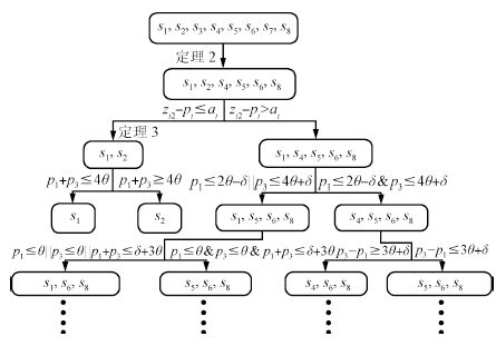
根据定理2 $\sim$ 4,结合单晶圆类型调度的全局搜索算法,首先利用驻留约束确定 $s_2$ 的可行性得到两个分枝,其中的第一分枝利用定理2和定理3里的支配关系排除了 $s_4$ , $s_5$ , $s_6$ , $s_7$ , $s_8$ ,第二分枝利用定理4的条件分析再进行分枝.图 2为改进型搜索决策树示例.
5. 实验分析
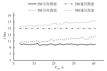
为了对带缓冲的集束型设备进行评价,把不带缓冲的集束型设备用于对比分析. 运用量化的分析方法,为带有缓冲的单臂集束型设备相对于无缓冲的集束型设备的产能提高提供了较为可靠的数据.本节中假设 $\delta=4$ , $\theta=2$ , $a_i=5$ 为最基本的实验条件.由于增加缓冲的优势主要体现在最大加工时间的加工模块上,所以有 $p_{\max}=\max_{1\leq i\leq 2m}\{p_i\}$ .用C++分别对两种算法进行编程,统计50组算例数据,求得平均的结果,并对比两种算法的数值实验结果. 图 3为两种算法所需的时间,可以看出分枝搜索的速度会比全局搜索算法更加优越.但图 4表明在小规模时,两种算法都能得到较好的结果.
将本文提出的算法与文献[13]的算法进行比较. 取加工时间为 $p_i\sim{\rm N}(60,2.5^2) $ ,如图 5所示为算法之间调度结果的比较.
由图 5可知,在小规模问题时,本文的算法与文献的算法得到的解基本相同,但随着规模的增加,本文的算法呈现出较为明显的优势,得到的解更优.
本文定义了提高率 $R$ 来评价带缓冲模块相对于无缓冲模块的系统之间产量提高:
$R=\frac{C{{T}_{G}}-C{{T}_{B}}}{C{{T}_{B}}}\times 100\%$
上式表示的是带缓冲的集束型设备与无缓冲的设备的集束型设备产能的提高率.其中 $R$ 越大,表示提高率越大.其中 $CT_B$ 代表带缓冲的集束型设备的周期时间,而 $CT_G$ 为无缓冲的集束型设备的周期时间. $Bd={p_{\max}}/{(\delta+\theta)}$ 表示搬运模块的繁忙程度, $Bd$ 越大表示搬运块模块越空闲.
5.1 生产率的提高与机械手的繁忙程度的关系
令机械手繁忙程度 $Bd$ 取[0,10]的均匀分布,通过仿真分析,得到如图 6的结果.
 图 6 生产率提高与搬运模块繁忙程度的关系Fig. 6 The relationship of improvement rates with the busy degree of TM
分析图 6可知,对于两集束型而言,仅当 $Bd\geq3$ 时,产能的提高率为正数,即仅当搬运模块繁忙程度 $Bd\geq3$ 时,缓冲模块能提高集束型设备的产能. 相反,当搬运模块繁忙程度 $Bd\leq3$ 时,产能提高率小于零,说明缓冲模块不提高产能,而对于三集束型而言, $Bd$ 的临界值为 $3.1$ .同时随着产能提高率的减少,最大加工时间 $p_{\max}$ 也相应减少,故TM在PM上等待时间也相应减少,直到晶圆加工完毕.若晶圆在PM上的等待搬运的时间大于驻留约束,那么搬运模块的搬运模式必须改变; 否则,晶圆会出现质量问题.无论搬运模块的繁忙程度如何的变化,最后TM都会处于搬运模式 $s_1$ ,说明在缓冲模块上的晶圆增加了额外的搬运.
5.2 生产率的提高与加工模块的加工时间的关系
设置变量 $P={p_t}/{(\delta+\theta)}$ ,然后令 $Bd$ 分布取均匀分布[3, 9]. 经过仿真分析,得到结果如图 7所示.
 图 7 生产率提高与加工时间之间的关系Fig. 7 The relationship of improvement rates with processing time of PMs
由图 7可知,在所有的搬运模块繁忙程度中,产能提高率从不稳定改变到达稳定的状态.主要原因在于随着模块加工时间的增加,搬运模块空闲使得加工模块的驻留约束的影响被降低.
6. 结论
本文针对带缓冲模块的集束型设备的调度问题建立了数学模型,构建全局搜索算法. 再通过具体分析两集束型设备,提出了分枝搜索算法.最后经仿真表明,分枝搜索算法比全局搜索算法更加迅速.同时通过和文献[13]的调度算法进行对比,表明本文的算法在加工模块比较少的时候调度结果提高不多,但随着规模增大,本文所得到的结果有明显的优势.通过对比带缓冲的集束型设备与无缓冲的集束型设备,证明了在加工模块之间增加缓冲,在一定程度上可以提高单臂集束型设备的产能.基于实验数据,仅当搬运模块TM的繁忙程度 $Bd$ 大于阈值时,设备产能才会提高.实验还表明驻留约束对于产能提高的影响是通过约束限制状态的改变产生的.随着加工模块的加工时间不断增加,产能提高越来越不显著,系统产能渐渐趋于平稳状态.
-
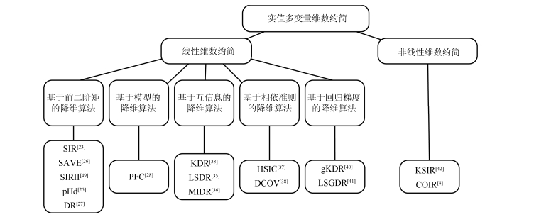
图 1 实值多变量维数约简算法分类
Fig. 1 Taxonomy of real-valued multivariate dimension reduction algorithms
表 1 基于互信息的降维算法对比
Table 1 Comparison of mutual information-based dimension reduction algorithms
目标函数 条件独立性 代表方法 解释 $\min_{{B}} {\rm E}_U \left[\mathbb{I}({Y|U};{V|U}) \right]$ ${Y}╨{V}|{U}$ KDR[32-33] 去掉$X$中与$Y$独立的一些特征, 也就是说这些特征对$Y$的预测不提供任何信息 $\max_{{B}} \mathbb{I}({Y};{U})$ ${Y}╨{X}|{U}$ LSDR[34-35]、MIDR[36] 从与$Y$相关的因素中寻找一个小的子空间或者子集, 不属于该子空间或者子集的特征, 虽然对$Y$的预测作出贡献, 但是在给定子空间或者子集后, 这部分信息不足以增加或改进对$Y$的预测能力  下载: 导出CSV
表 2 实值多变量维数约简算法总结
Table 2 Summary of real-valued multivariate dimension reduction algorithms
算法 响应变量 求解类型 分布假设 统计矩 模型选取 回归方式 #参数 参数列表 SIR[23] 一元 解析解 椭圆对称 一阶 无 逆回归 1 切片数$h$ SAVE[26] 一元 解析解 椭圆对称 二阶 无 逆回归 1 $h$ SIRII[49] 一元 解析解 椭圆对称 二阶 无 逆回归 1 $h$ pHd[25] 一元 解析解 正态分布 二阶 - 正回归 0 - DR[27] 一元 解析解 渐进正态 二阶 无 逆回归 1 $h$ PFC[28] 一元 解析解 模型假设 模型相关 无 逆回归 1 次数$r$ KDR[33] 多元 非凸优化 无 无穷 无 正回归 3 带宽$\sigma_x, \sigma_y$, $\epsilon$ LSDR[35] 多元 非凸优化 无 无穷 交叉验证 正回归 4 $\sigma_x, \sigma_y$, $\lambda$, $b$ MIDR[36] 多元 非凸优化 无 无穷 - 正回归 0 - HSIC[37] 多元 非凸优化 无 无穷 无 正回归 2 $\sigma_x, \sigma_y$ DCOV[38] 多元 非凸优化 无 二阶 - 正回归 0 - gKDR[40] 多元 解析解 无 无穷 无 正回归 3 $\sigma_x, \sigma_y, \epsilon$ LSGDR[41] 多元 解析解 无 无穷 交叉验证 正回归 $2D+1$ $\{\sigma_x^{(j)}, \lambda^{(j)}\}_{j=1}^D, \sigma_y$ KSIR[42] 一元 解析解 无 无穷 无 逆回归 2 $\sigma_x$, $h$ COIR[8] 多元 解析解 无 无穷 无 逆回归 3 $\sigma_x, \sigma_y, \epsilon$
下载: 导出CSV
表 3 基于广义特征值求解的实值多变量维约简算法估计量
Table 3 Estimation of generalized eigen-decomposition-based multivariate dimension reduction algorithms
方法 (样本)估计量${M}$ SIR[23] ${\rm E}\Big[{\rm E}(Z|Y){\rm E}(Z|Y)^{\rm T}\Big] $ SAVE[26] ${\rm E}\Big[{I}-{\rm var}(Z|Y)\Big]^2$ SIRII[49] ${\rm E}\Big[{\rm var}(Z|Y)-{\rm E}({\rm var}(Z|Y))\Big]^2$ pHd[25] ${\rm E}\Big[(Y-E Y)ZZ^{\rm T}\Big]^2$ DR[27] $2{\rm E}\Big[E^2(ZZ^{\rm T}|Y)\Big]+ 2E^2\Big[{\rm E}(Z|Y){\rm E}(Z^{\rm T}|Y)\Big]+$ $ 2{\rm E}\Big[{\rm E}(Z^{\rm T}|Y){\rm E}(Z|Y)\Big]{\rm E}\Big[{\rm E}(Z|Y) {\rm E}(Z^{\rm T}|Y)\Big]\!-\!2{I}$ PFC[28] $\frac{1}{n}\widehat{{X}}^{\rm T}\widehat{{X}}$ gKDR[40] $ \big\langle \frac{\partial \kappa_x(\cdot, {\pmb x})}{\partial {\pmb x}}, \Sigma_{XX}^{-1}\Sigma_{XY}\Sigma_{YX}\Sigma_{XX}^{-1}\frac{\partial \kappa_x(\cdot, {\pmb x})}{\partial {\pmb x}}\big\rangle_{\mathcal{H}_x}$ LSGDR[41] $ {\rm E}({{\pmb g}}(y, {\pmb x}){{\pmb g}}(y, {\pmb x})^{\rm T})$ KSIR[42] ${\rm var}({\rm E}[{ \pmb \phi}({\pmb x})|y])$ COIR[8] ${\rm var}({\rm E}[{ \pmb \phi}({\pmb x})|y])$
下载: 导出CSV
表 4 通过矩阵流形优化的降维算法的总结
Table 4 Summary of matrix manifold optimization-based dimension reduction algorithms
算法 目标函数$f({B})$ 欧式空间梯度$\nabla_{{B}} f$ 对应的权值矩阵${W}$ KDR[33] ${\rm{tr}}[{\overline{K}}_Y({\overline{K}}_U+n\epsilon {I}_n)^{-1}]$ $\frac{2}{\sigma^2}{X}{L}_{{\rm{KDR}}}{X}^{\rm T}{B}$ $\begin{array}{rl} {W}_{hrm{KDR}} &\!\!\!\!\!\!\!={H}{\Omega}{H}\odot{K}_U\\ {\Omega} &\!\!\!\!\!\!\!= {M}^{-1}{H}{K}_Y{H}{M}^{-1} \\ {M} &\!\!\!\!\!\!\!= {H}{K}_U{H}+n \epsilon {I} \end{array}$ LSDR[35] $\frac{1}{2}{\hat{\pmb{\alpha}}}^{\rm T}{\widehat{H}}{\hat{\pmb{\alpha}}}- \widehat{\pmb{h}}^{\rm T}\widehat{\pmb{\alpha}}$ 不存在解析形式梯度 无拉普拉斯形式 MIDR[36] $\begin{array}{ll}&\frac{d+1}{n(n-1)}\sum_{i\neq j}\log(\left\| {({\pmb x}_i- {\pmb x}_j){B}} \right\|^2+\left\| {y_i-y_j} \right\|^2)-\\ &\frac{d}{n(n-1)}\sum_{i\neq j}\log\left\| {({\pmb x}_i-{\pmb x}_j){B}} \right\| ^2\end{array}$ $-\frac{4}{n(n-1)} {X}{L}_{{\rm{MIDR}}}{X}^{\rm T}{B}$ $\begin{array}{rl}&{W}_{hrm{MIDR}}=\frac{d}{{D}_X\!\odot\!{D}_X}- \\ &\frac{d+1}{({D}_X\!\odot\!{D}_X\!+\!{D}_Y\!\odot\!{D}_Y)}\end{array}$ HSIC[37] $-\frac{1}{(n-1)^2}\textrm{tr}\big[{K}_U{H}{K}_Y {H}\big]$ $\frac{2}{\sigma^2(n-1)^2}{X}{L}_{{\rm{HSIC}}}{X}^{\rm T}{B}$ ${W}_{{\rm{HSIC}}} = {H}{K}_Y{H}\odot{K}_U$ DCOV[38] $-\frac{1}{n^2}{\rm{tr}}\big[{\overline{D}}_U{\overline{D}}_Y\big]$ $-\frac{2}{n^2}{X}{L}_{{\rm{DCOV}}}{X}^{\rm T}{B}$ ${W}_{{\rm{DCOV}}} = \frac{{H}{D}_Y{H}}{{D}_U}$
下载: 导出CSV
-
[1] Jolliffe I. Principal Component Analysis. New York:Wiley Online Library, 2002. [2] Hotelling H. Analysis of a complex of statistical variables into principal components. Journal of Educational Psychology, 1993, 24 (6):417-441 http://www.docin.com/p-238815088.html [3] Roweis S T, Saul L K. Nonlinear dimensionality reduction by locally linear embedding. Science, 2000, 290 (5500):2323-2326 doi: 10.1126/science.290.5500.2323 [4] Tenenbaum J B, Silva V D, Langford J C. A global geometric framework for nonlinear dimensionality reduction. Science, 2000, 290 (5500):2319-2323 doi: 10.1126/science.290.5500.2319 [5] Fisher R A. The use of multiple measurements in taxonomic problems. Annals of Eugenics, 1936, 7 (2):179-188 https://www.bibsonomy.org/bibtex/2c9d8d78a8e1bb5adecc7602490f4323f/gromgull [6] Mika S, Ratsch G, Weston J, Schölkopft B, Mullert K R. Fisher discriminant analysis with kernels. In: Proceeding of the 1999 IEEE Signal Processing Society on Neural Networks for Signal Processing Ⅸ. Madison, WI, USA, USA: IEEE, 1999. 41-48 http://ieeexplore.ieee.org/xpls/abs_all.jsp?arnumber=788121 [7] Kulis B. Metric learning:a survey. Foundations and Trends in Machine Learning, 2012, 5 (4):287-364 https://www.cs.cmu.edu/~liuy/frame_survey_v2.pdf [8] Kim M, Pavlovic V. Central subspace dimensionality reduction using covariance operators. IEEE Transactions on Pattern Analysis and Machine Intelligence, 2011, 33 (4):657-670 doi: 10.1109/TPAMI.2010.111 [9] Tan B, Zhang J P, Wang L. Semi-supervised elastic net for pedestrian counting. Pattern Recognition, 2011, 44 (10-11):2297-2304 doi: 10.1016/j.patcog.2010.10.002 [10] Zhang J P, Tan B, Sha F, He L. Predicting pedestrian counts in crowded scenes with rich and high-dimensional features. IEEE Transactions on Intelligent Transportation Systems, 2011, 12 (4):1037-1046 https://www.researchgate.net/profile/Junping_Zhang/publication/220109419_Predicting_Pedestrian_Counts_in_Crowded_Scenes_With_Rich_and_High-Dimensional_Features/links/0deec53b629366a5b6000000.pdf?inViewer=true&pdfJsDownload=true&disableCoverPage=true&origin=publication_detail [11] Kim M Y, Pavlovic V. Dimensionality reduction using covariance operator inverse regression. In: Proceedings of the 2008 IEEE Conference on Computer Vision and Pattern Recognition. Anchorage, AK, USA: IEEE, 2008. 1-8 http://ieeexplore.ieee.org/xpls/abs_all.jsp?arnumber=4587404 [12] Zhang J P, Wang F Y, Wang K F, Lin W H, Xu X, Chen C. Data-driven intelligent transportation systems:a survey. IEEE Transactions on Intelligent Transportation Systems, 2011, 12 (4):1037-1046 doi: 10.1109/TITS.2011.2132759 [13] Zhu H J, Li L X. Biological pathway selection through nonlinear dimension reduction. Biostatistics, 2011, 12 (3):429-444 doi: 10.1093/biostatistics/kxq081 [14] Zhu H J, Li L X, Zhou H. Nonlinear dimension reduction with Wright-Fisher kernel for genotype aggregation and association mapping. Bioinformatics, 2012, 28 (18):i375-i381 doi: 10.1093/bioinformatics/bts406 [15] Shan H M, Zhang J P, Kruger U. Learning linear representation of space partitioning trees based on unsupervised kernel dimension reduction. IEEE Transactions on Cybernetics, 2016, 46 (12):3427-3438 doi: 10.1109/TCYB.2015.2507362 [16] Bishop C M. Pattern Recognition and Machine Learning. New York:Springer, 2006. [17] Caruana R. Multitask learning. Machine Learning, 1997, 28 (1):41-75 doi: 10.1023/A:1007379606734 [18] Tsoumakas G, Katakis I. Multi-label classification:an overview. International Journal of Data Warehousing and Mining, 2007, 3 (3):1-13 doi: 10.4018/IJDWM [19] Tipping M E. Sparse Bayesian learning and the relevance vector machine. Journal of Machine Learning Research, 2001, 1:211-244 https://dl.acm.org/citation.cfm?id=944741 [20] 王卫卫, 李小平, 冯象初, 王斯琪.稀疏子空间聚类综述.自动化学报, 2015, 41 (8):1373-1384 http://www.aas.net.cn/CN/abstract/abstract18712.shtmlWang Wei-Wei, Li Xiao-Ping, Feng Xiang-Chu, Wang Si-Qi. A survey on sparse subspace clustering. Acta Automatica Sinica, 2015, 41 (8):1373-1384 http://www.aas.net.cn/CN/abstract/abstract18712.shtml [21] Koller D, Friedman N. Probabilistic Graphical Models:Principles and Techniques. Massachusetts:MIT Press, 2009. [22] 刘建伟, 黎海恩, 罗雄麟.概率图模型学习技术研究进展.自动化学报, 2014, 40 (6):1025-1044 http://www.aas.net.cn/CN/abstract/abstract18373.shtmlLiu Jian-Wei, Li Hai-En, Luo Xiong-Lin. Learning technique of probabilistic graphical models:a review. Acta Automatica Sinica, 2014, 40 (6):1025-1044 http://www.aas.net.cn/CN/abstract/abstract18373.shtml [23] Li K C. Sliced inverse regression for dimension reduction. Journal of the American Statistical Association, 1991, 86 (414):316-327 doi: 10.1080/01621459.1991.10475035 [24] Chiaromonte F, Cook R D. Sufficient dimension reduction and graphics in regression. Annals of the Institute of Statistical Mathematics, 2002, 54 (4):768-795 doi: 10.1023/A:1022411301790 [25] Li K C. On principal Hessian directions for data visualization and dimension reduction:another application of Stein's lemma. Journal of the American Statistical Association, 1992, 87 (420):1025-1039 doi: 10.1080/01621459.1992.10476258 [26] Cook R D, Weisberg S. Sliced inverse regression for dimension reduction:comment. Journal of the American Statistical Association, 1991, 86 (414):328-332 http://citeseerx.ist.psu.edu/showciting?cid=2673643 [27] Li B, Wang S L. On directional regression for dimension reduction. Journal of the American Statistical Association, 2007, 102 (479):997-1008 doi: 10.1198/016214507000000536 [28] Cook R D. Fisher lecture:dimension reduction in regression. Statistical Science, 2007, 22 (1):1-26 doi: 10.1214/088342306000000682 [29] Cook R D, Forzani L. Principal fitted components for dimension reduction in regression. Statistical Science, 2008, 23 (4):485-501 doi: 10.1214/08-STS275 [30] Cook R D, Forzani L. Likelihood-based sufficient dimension reduction. Journal of the American Statistical Association, 2009, 104 (485):197-208 doi: 10.1198/jasa.2009.0106 [31] Bach F R, Jordan M I. Kernel independent component analysis. Journal of Machine Learning Research, 2002, 3:1-48 [32] Fukumizu K, Bach F R, Jordan M I. Dimensionality reduction for supervised learning with reproducing kernel Hilbert spaces. Journal of Machine Learning Research, 2004, 5:73-99 http://www.ams.org/mathscinet-getitem?mr=2247974 [33] Fukumizu K, Bach F R, Jordan M I. Kernel dimension reduction in regression. The Annals of Statistics, 2009, 37 (4):1871-1905 doi: 10.1214/08-AOS637 [34] Suzuki T, Sugiyama M. Sufficient dimension reduction via squared-loss mutual information estimation. In Proceedings of International Conference on Artificial Intelligence and Statistics, Chia Laguna Resort, Sardinia, Italy, 2010, 9:804-811 https://www.researchgate.net/profile/Masashi_Sugiyama/publication/220320963_Sufficient_Dimension_Reduction_via_Squared-loss_Mutual_Information_Estimation/links/0fcfd51196d6b08046000000.pdf?origin=publication_detail [35] Suzuki T, Sugiyama M. Sufficient dimension reduction via squared-loss mutual information estimation. Neural Computation, 2013, 25 (3):725-758 doi: 10.1162/NECO_a_00407 [36] Faivishevsky L, Goldberger J. Dimensionality reduction based on non-parametric mutual information. Neurocomputing, 2012, 80:31-37 doi: 10.1016/j.neucom.2011.07.028 [37] Wang M H, Sha F, Jordan M I. Unsupervised kernel dimension reduction. In: Proceedings of the Advances in Neural Information Processing Systems. Vancouver, Canada, 2010. 2379-2387 [38] Sheng W H, Yin X R. Sufficient dimension reduction via distance covariance. Journal of Computational and Graphical Statistics, 2016, 25 (1):91-104 doi: 10.1080/10618600.2015.1026601 [39] Fukumizu K, Leng C L. Gradient-based kernel method for feature extraction and variable selection. In: Proceedings of the Advances in Neural Information Processing Systems. Lake Tahoe, Nevada, 2012. 2114-2122 https://www.researchgate.net/publication/287550602_Gradient-based_kernel_method_for_feature_extraction_and_variable_selection [40] Fukumizu K, Leng C L. Gradient-based kernel dimension reduction for regression. Journal of the American Statistical Association, 2014, 109 (505):359-370 doi: 10.1080/01621459.2013.838167 [41] Sasaki H, Tangkaratt V, Sugiyama M. Sufficient dimension reduction via direct estimation of the gradients of logarithmic conditional densities. In: Proceedings of the 7th Asian Conference on Machine Learning. Hong Kong, China: PMLR, 2015. 33-48 http://europepmc.org/abstract/MED/29162006 [42] Wu H M. Kernel sliced inverse regression with applications to classification. Journal of Computational and Graphical Statistics, 2012, 17 (3):590-610 doi: 10.1198/106186008X345161 [43] Li L X. Sparse sufficient dimension reduction. Biometrika, 2007, 94 (3):603-613 doi: 10.1093/biomet/asm044 [44] Chen X, Zou C L, Cook R D. Coordinate-independent sparse sufficient dimension reduction and variable selection. The Annals of Statistics, 2010, 38 (6):3696-723 doi: 10.1214/10-AOS826 [45] Nilsson J, Sha F, Jordan M I. Regression on manifolds using kernel dimension reduction. In: Proceedings of the 24th International Conference on Machine Learning. Corvalis, Oregon, USA: ACM, 2007. 697-704 http://dl.acm.org/citation.cfm?id=1273584 [46] Shyr A, Urtasun R, Jordan M I. Sufficient dimension reduction for visual sequence classification. In: Proceedings of the 2010 IEEE Conference on Computer Vision and Pattern Recognition. San Francisco, California, USA: IEEE, 2010. 3610-3617 http://ieeexplore.ieee.org/xpls/icp.jsp?arnumber=5539922 [47] Cook R D. On the interpretation of regression plots. Journal of the American Statistical Association, 1994, 89 (425):177-189 doi: 10.1080/01621459.1994.10476459 [48] Cook R D. Using dimension-reduction subspaces to identify important inputs in models of physical systems. In: Proceedings of the Section on Physical and Engineering Sciences. 1994. 18-25 https://www.researchgate.net/publication/313634045_Using_dimension-reduction_subspaces_to_identify_important_inputs_in_models_of_physical_systems [49] Li K C. Sliced inverse regression for dimension reduction:rejoinde. Journal of the American Statistical Association, 1991, 86 (414):337-342 [50] Harrison D, Rubinfeld D L. Hedonic housing prices and the demand for clean air. Journal of Environmental Economics and Management, 1978, 5 (1):81-102 https://ideas.repec.org/r/eee/jeeman/v5y1978i1p81-102.html [51] Stein C M. Estimation of the mean of a multivariate normal distribution. The Annals of Statistics, 1981, 9 (6):1135-1151 doi: 10.1214/aos/1176345632 [52] Li K C, Lue H H, Chen C H. Interactive tree-structured regression via principal Hessian directions. Journal of the American Statistical Association, 2000, 95 (450):547-560 doi: 10.1080/01621459.2000.10474231 [53] Gannoun A, Saracco J. An asymptotic theory for SIR α method. Statistica Sinica, 2003, 13:297-310 https://www.researchgate.net/publication/265359288_An_asymptotic_theory_for_SIR_a_method [54] Ye Z S, Weiss R E. Using the bootstrap to select one of a new class of dimension reduction methods. Journal of the American Statistical Association, 2003, 98 (464):968-979 doi: 10.1198/016214503000000927 [55] Li B, Zha H Y, Chiaromonte F. Contour regression:a general approach to dimension reduction. The Annals of Statistics, 2005, 33 (4):1580-1616 doi: 10.1214/009053605000000192 [56] Tipping M E, Bishop C M. Probabilistic principal component analysis. Journal of the Royal Statistical Society:Series B (Statistical Methodology), 1999, 61 (3):611-622 doi: 10.1111/rssb.1999.61.issue-3 [57] Cook R D, Forzani L M, Tomassi D R. LDR:a package for likelihood-based sufficient dimension reduction. Journal of Statistical Software, 2011, 39 (3):1-20 https://www.researchgate.net/profile/Kofi_Adragni/publication/279335077_ldr_An_R_Software_Package_for_Likelihood-Based_Sufficient_Dimension_Reduction/links/578c764208ae59aa667c5320/ldr-An-R-Software-Package-for-Likelihood-Based-Sufficient-Dimension-Reduction.pdf [58] Baker C R. Joint measures and cross-covariance operators. Transactions of the American Mathematical Society, 1973, 186:273-289 doi: 10.1090/S0002-9947-1973-0336795-3 [59] Absil P A, Mahony R, Sepulchre R. Optimization Algorithms on Matrix Manifolds. Princeton:Princeton University Press, 2009. [60] Zhang K, Tsang I W, Kwok J T. Improved Nystr öm low-rank approximation and error analysis. In: Proceedings of the 25th International Conference on Machine Learning. Helsinki, Finland: ACM, 2008. 1232-1239 http://dl.acm.org/citation.cfm?id=1390311 [61] Sugiyama M, Suzuki T, Kanamori T. Density Ratio Estimation in Machine Learning. Cambridge:Cambridge University Press, 2012. [62] Nguyen X, Wainwright M J, Jordan M I. Estimating divergence functionals and the likelihood ratio by penalized convex risk minimization. In: Proceedings of the Advances in Neural Information Processing Systems. Vancouver, Canada: ACM, 2008. 1089-1096 [63] Yamada M, Niu G, Takagi G, Sugiyama M. Computationally efficient sufficient dimension reduction via squared-loss mutual information. In: Proceedings of the 3rd Asian Conference on Machine Learning. Canberra, Australia: ACML, 2011. 247-262 https://www.researchgate.net/publication/215705073_Computationally_Efficient_Sufficient_Dimension_Reduction_via_Squared-Loss_Mutual_Information?ev=auth_pub [64] Faivishevsky L, Goldberger J. ICA based on a smooth estimation of the differential entropy. In: Proceedings of the Advances in Neural Information Processing Systems. Vancouver, British Columbia, Canada: ACM, 2009. 433-440 https://www.researchgate.net/publication/221618225_ICA_based_on_a_Smooth_Estimation_of_the_Differential_Entropy [65] Faivishevsky L, Goldberger J. Nonparametric information theoretic clustering algorithm. In: Proceedings of the 27th International Conference on Machine Learning. Haifa, Israel: ICML, 2010. 351-358 [66] Loftsgaarden D O, Quesenberry C P. A nonparametric estimate of a multivariate density function. The Annals of Mathematical Statistics, 1965, 36 (3):1049-1051 doi: 10.1214/aoms/1177700079 [67] Gretton A, Smola A J, Bousquet O, Herbrich R, Belitski A, Augath M, Murayama Y, Pauls J, Sch ölkopf B, Logothetis N K. Kernel constrained covariance for dependence measurement. In: Proceedings of the 10th International Workshop on Artificial Intelligence and Statistics. Barbados, 2005. 1-8 https://www.researchgate.net/publication/41781419_Kernel_Constrained_Covariance_for_Dependence_Measurement [68] Gretton A, Bousquet O, Smola A, Sch ölkopf B. Measuring statistical dependence with Hilbert-Schmidt norms. In: Proceedings of the 16th International Conference on Algorithmic Learning Theory. Berlin, Heidelberg: Springer-Verlag, 2005. 63-77 doi: 10.1007/11564089_7 [69] Sz ékely G J, Rizzo M L, Bakirov N K. Measuring and testing dependence by correlation of distances. The Annals of Statistics, 2007, 35 (6):2769-2794 doi: 10.1214/009053607000000505 [70] Zhang Y, Zhou Z H. Multi-label dimensionality reduction via dependence maximization. ACM Transactions on Knowledge Discovery from Data, 2010, 4 (3):Article No.14 https://cs.nju.edu.cn/zhouzh/zhouzh.files/publication/tkdd10mddm.pdf [71] Song L, Smola A, Gretton A, Borgwardt K M. A dependence maximization view of clustering. In: Proceedings of the 24th International Conference on Machine Learning. Corvalis, Oregon, USA: ACM, 2007. 815-822 http://dl.acm.org/citation.cfm?id=1273599 [72] Blaschko M, Gretton A. Learning taxonomies by dependence maximization. In: Proceedings of the Advances in Neural Information Processing Systems. Vancouver, B. C., Canada, 2009. 153-160 https://www.researchgate.net/publication/41782196_Learning_Taxonomies_by_Dependence_Maximization [73] Song L, Smola A, Gretton A, Bedo J, Borgwardt K. Feature selection via dependence maximization. The Journal of Machine Learning Research, 2012, 13 (1):1393-1434 https://dl.acm.org/citation.cfm?id=2343691 [74] Quadrianto N, Song L, Smola A J. Kernelized sorting. In: Proceedings of the Advances in neural information processing systems. Vancouver, B. C., Canada, 2009. 1289-1296 [75] Quadrianto N, Smola A J, Song L, Tuytelaars T. Kernelized sorting. IEEE Transactions on Pattern Analysis and Machine Intelligence, 2010, 32 (10):1809-1821 doi: 10.1109/TPAMI.2009.184 [76] Sun X H, Janzing D, Sch ölkopf B, Fukumizu K. A kernel-based causal learning algorithm. In: Proceedings of the 24th International Conference on Machine Learning. Corvalis, Oregon, USA: ACM, 2007. 855-862 [77] Li R Z, Zhong W, Zhu L P. Feature screening via distance correlation learning. Journal of the American Statistical Association, 2012, 107 (499):1129-1139 doi: 10.1080/01621459.2012.695654 [78] Vepakomma P, Tonde C, Elgammal A. Supervised dimensionality reduction via distance correlation maximization. arXiv: 1601. 00236, 2016. http://arxiv.org/abs/1601.00236 [79] Sz ékely G J, Rizzo M L. Brownian distance covariance. The Annals of Applied Statistics, 2009, 3 (4):1236-1265 doi: 10.1214/09-AOAS312 [80] Sejdinovic D, Sriperumbudur B, Gretton A, Fukumizu K. Equivalence of distance-based and RKHS-based statistics in hypothesis testing. The Annals of Statistics, 2013, 41 (5):2263-2291 doi: 10.1214/13-AOS1140 [81] Fukumizu K, Gretton A, Sun X H, Sch ölkopf B. Kernel measures of conditional dependence. In: Proceedings of the Advances in Neural Information Processing Systems. Vancouver, British Columbia, Canada: Curran Associates Inc., 2007. 489-496 [82] P óczos B, Ghahramani Z, Schneider J G. Copula-based kernel dependencymeasures. In: Proceedings of the 29th International Conference on Machine Learning. Edinburgh, Scotland: ICML, 2012. 1635-1642 http://www.oalib.com/paper/4033144 [83] Schweizer B, Wolff E F. On nonparametric measures of dependence for random variables. The Annals of Statistics, 1981, 9 (4):879-885 doi: 10.1214/aos/1176345528 [84] Steinwart I, Christmann A. Support Vector Machines. Berlin, Heidelberg:Springer Science & Business Media, 2008. [85] Kim M Y, Pavlovic V. Covariance operator based dimensionality reduction with extension to semi-supervised settings. In: Proceedings of the 12th International Conference on Artificial Intelligence and Statistics. Varna, Bulgaria: Springe, 2009. 280-287 https://www.researchgate.net/publication/220319841_Covariance_Operator_Based_Dimensionality_Reduction_with_Extension_to_Semi-Supervised_Settings [86] Zou H, Hastie T, Tibshirani R. Sparse principal component analysis. Journal of Computational and Graphical Statistics, 2006, 15 (2):265-286 doi: 10.1198/106186006X113430 [87] Cunningham J P, Ghahramani Z. Linear dimensionality reduction:Survey, insights, and generalizations. Journal of Machine Learning Research, 2015, 16:2859-2900 https://arxiv.org/abs/1406.0873 [88] Fan K, Hoffman A J. Some metric inequalities in the space of matrices. Proceedings of the American Mathematical Society, 1995, 6 (1):111-116 doi: 10.1142/9789812796936_0012 [89] Kaneko T, Fiori S, Tanaka T. Empirical arithmetic averaging over the compactStiefel manifold. IEEE Transactions on Signal Processing, 2013, 61 (4):883-894 doi: 10.1109/TSP.2012.2226167 [90] Cook R D, Yin X R. Theory & methods:special invited paper:dimension reduction and visualization in discriminant analysis (with discussion). Australian & New Zealand Journal of Statistics, 2001, 43 (2):147-199 doi: 10.1146/annurev.psych.52.1.1 [91] Zhu Y, Zeng P. Fourier methods for estimating the central subspace and the central mean subspace in regression. Journal of the American Statistical Association, 2006, 101 (476):1638-1651 doi: 10.1198/016214506000000140 [92] Davies A C, Yin J H, Velastin S A. Crowd monitoring using image processing. Electronics & Communication Engineering Journal, 1995, 7 (1):37-47 https://www.researchgate.net/publication/3364407_Crowd_monitoring_using_image_processing [93] Cho S Y, Chow T W, Leung C T. A neural-based crowd estimation by hybrid global learning algorithm. IEEE Transactions on Systems, Man, and Cybernetics, Part B (Cybernetics), 1999, 29 (4):535-541 doi: 10.1109/3477.775269 [94] 时增林, 叶阳东, 吴云鹏, 娄铮铮.基于序的空间金字塔池化网络的人群计数方法.自动化学报, 2016, 42(6):866-874 http://www.aas.net.cn/CN/abstract/abstract18877.shtmlShi Zeng-Lin, Ye Yang-Dong, Wu Yun-Peng, Lou Zheng-Zheng. Crowd counting using rank-based spatial pyramid pooling network. Acta Automatica Sinica, 2016, 42 (6):866-874 http://www.aas.net.cn/CN/abstract/abstract18877.shtml [95] Dasgupta S, Freund Y. Random projection trees and low dimensional manifolds. In: Proceedings of the 40th Annual ACM Symposium on Theory of Computing. Victoria, British Columbia, Canada: ACM, 2008. 537-546 http://dl.acm.org/citation.cfm?id=1374452 期刊类型引用(6)
1. 黄年昌,杨阳,张强,韩军功. 基于深度学习的RGB-D图像显著性目标检测前沿进展. 计算机学报. 2025(02): 284-316 .  百度学术
百度学术2. 闫梦凯,钱建军,杨健. 弱对齐的跨光谱人脸检测. 自动化学报. 2023(01): 135-147 . 本站查看3. 王利锋,辛丽平,刘家硕,鞠莲. 基于热红外视频图像监测的海面溢油识别技术研究. 海洋学报. 2022(05): 148-160 . 百度学术4. 蔺素珍,张海松,禄晓飞,李大威,李毅. RBNSM:一种复杂背景下红外弱小目标检测新方法. 红外技术. 2022(07): 667-675 . 百度学术5. 刘晓玲,牛海春,宋海燕,秦富贞. 复杂环境下弱信号中的红外小目标自动检测. 激光杂志. 2020(10): 82-86 . 百度学术6. 刘松涛,姜康辉,刘振兴. 基于区域协方差和目标度的航空侦察图像舰船目标检测. 系统工程与电子技术. 2019(05): 972-980 . 百度学术其他类型引用(2)
-


 下载:
下载:


计量
- 文章访问数: 3317
- HTML全文浏览量: 398
- PDF下载量: 1482
- 被引次数: 8
