

-
摘要: 相机全局位置估计作为运动恢复结构算法(Structure from motion,SfM)中的核心内容一直以来都是计算机视觉领域的研究热点.现有相机全局位置估计方法大多对外点敏感,在处理大规模、无序图像集时表现的尤为明显.增量式SfM中的迭代优化步骤可以剔除大部分的误匹配从而降低外点对估计结果的影响,而全局式SfM中没有有效地剔除误匹配的策略,估计结果受外点影响较大.针对这种情况,本文提出一种改进的相机全局位置估计方法:首先,结合极线约束提出一种新的对误匹配鲁棒的相对平移方向估计算法,减少相对平移方向估计结果中存在的外点;然后,引入平行刚体理论提出一种新的预处理方法将相机全局位置估计转化为一个适定性问题;最后,在此基础上构造了一个对外点鲁棒的凸优化线性估计模型,对模型解算获取相机位置估计全局最优解.本文方法可以很好地融合到当下的全局式SfM流程中.与现有典型方法的对照实验结果表明:在处理大规模、无序图像时,本文方法能显著提高相机全局位置估计的鲁棒性,并保证估计过程的高效性和估计结果的普遍精度.Abstract: As a core module of structure from motion (SfM), location estimation of cameras in a global framework has been a research hotspot of computer version. State-of-the-art methods for location estimation are sensitive to outliers, especially for large scale, unordered images. The incremental SfM reduces the influence of outliers through an iterative optimization. The global SfM does not have an efficient strategy to remove mismatch, so the result of estimation is influenced deeply by outliers. Therefore, we introduce an improved method for location estimation. First, combined with the epipolar constraint we propose a new pairwise direction estimation algorithm. Then, we make the problem well-posed by introducing a new preprocessing method based on parallel rigidity. Finally, we propose a robust linear estimation model based on convex programing. We can get a global optimum solution by resolving this model. The method can integrate well with state-of-art global SfM pipeline. Multiple group experiments have proved the robustness of our methods without any loss of efficiency and common precision.1) 本文责任编委 贾云得
-

图 1 融合本文改进的全局式SfM算法流程图
Fig. 1 The processing pipeline of global SfM fusion our modifying

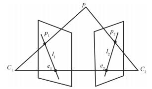
图 2 本文改进的相对平移方向估计算法流程
Fig. 2 The processing pipeline of relative translation estimation based on our modifying

图 11 利用本文算法对8组公开数据集处理获取的场景三维稀疏结构
Fig. 11 The experimental result with 8 groups of datasets based on our method
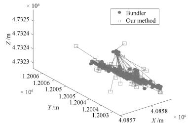
图 6 相机全局位置散点图(数据Vienna, 相机个数821)
Fig. 6 Global location of cameras represented by scatter diagram
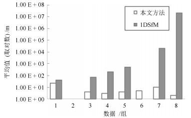
图 7 BA优化后本文同1DSfM实验结果平均值比较图
Fig. 7 Comparison result of mean between our method and 1DSfM after BA

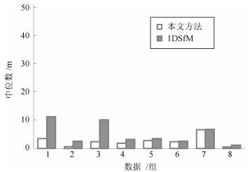
图 9 BA优化前本文同1DSfM实验结果中位数比较图
Fig. 9 Comparison result of median between our method and 1DSfM before BA
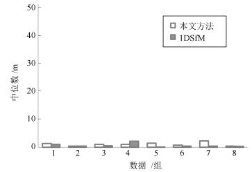
图 10 BA优化后本文同1DSfM实验结果中位数比较图
Fig. 10 Comparison result of median between our method and 1DSfM after BA
数据 本文方法 1DSfM [23] [20] 初始 BA后 初始 BA后 BA后 名称 尺寸(像素) 数目 $\widetilde{x}$ $\overline{x}$ $N$ $\widetilde{x}$ $\overline{x}$ $\widetilde{x}$ $N$ $\widetilde{x}$ $\overline{x}$ $N$ $\widetilde{x}$ Tower 1 600×1 064 1 576 3.4 19 461 1.3 22 11 414 1.0 40 306 44 Montreal 1 349×1 600 2 298 0.6 1 454 0.4 1 2.5 427 0.4 1 357 9.8 Madrid 1 600×1 081 1 344 2.3 5 337 1.0 4 9.9 291 0.5 70 240 18 Piazza 1 600×2 390 2 251 1.8 5 318 1.0 3 3.1 308 2.1 200 93 16 Yorkminster 1 600×2 129 3 368 2.7 6 406 1.4 4 3.4 401 0.1 500 345 6.7 Library 1 067×1 600 2 550 2.3 6 321 0.7 5 2.5 295 0.4 1 271 1.4 Vienna 1 600×2 400 6 288 6.5 16 821 2.2 10 6.6 770 0.4 2E4 652 12 Alamo 1 600×2 133 2 915 0.5 2 554 0.4 2 1.1 529 0.3 2E7 422 2.4  下载: 导出CSV
表 2 本文方法同1DSfM、文献[20]、Bundler处理时间比较
Table 2 Comparison of efficiency: our method、1DSfM、Bundler and [20]
数据 本文方法 1DSfM [23] [20] Bundler $T_R$ $T_O$ $T_S$ $T_{BA}$ $\Sigma$ $T_R$ $T_O$ $T_S$ $T_{BA}$ $\Sigma$ $\Sigma$ $\Sigma$ Tower 1 29 9 351 390 9 14 55 606 648 264 1 900 Montreal 2 66 24 352 444 17 22 75 1 135 1 249 424 2 710 Madrid 1 12 7 158 178 15 8 20 201 244 139 1 315 Piazza 1 14 11 95 121 14 9 35 191 249 138 1 287 Yorkminster 1 31 12 128 172 11 18 93 777 899 394 3 225 Library 1 13 6 199 219 9 13 54 392 468 220 3 807 Vienna 6 344 50 1 206 1 606 98 60 144 2 837 3 139 2 273 10 276 Alamo 4 153 49 847 1 053 56 29 73 752 910 1 403 1 654
下载: 导出CSV
-
[1] Triggs B, McLauchlan P, Hartley R I, Fitzgibbon A W. Bundle adjustment-a modern synthesis. Vision Algorithms: Theory and Practice: Lecture Notes in Computer Science. Berlin, Heidelberg: Springer, 1999. 298-372 doi: 10.1007/3-540-44480-7 [2] Zhang Z Y, Shan Y. Incremental Motion Estimation Through Local Bundle Adjustment. Technical Report MSR-TR-01-54, Microsoft Research, Redmond, WA, 2001. [3] Snavely N, Seitz S M, Szeliski R. Photo tourism:exploring photo collections in 3D. ACM Transactions on Graphics, 2006, 25(3):835-846 doi: 10.1145/1141911 [4] Snavely N, Seitz S M, Szeliski R. Skeletal graphs for efficient structure from motion. In: Proceedings of the 2008 IEEE Conference on Computer Vision and Pattern Recognition. Anchorage, USA: IEEE, 2008. 1-8 http://ieeexplore.ieee.org/xpls/icp.jsp?arnumber=4587678 [5] Havlena M, Torii A, Knopp J, Pajdla T. Randomized structure from motion based on atomic 3D models from camera triplets. In: Proceedings of the 2009 IEEE Conference on Computer Vision and Pattern Recognition. Miami, USA: IEEE, 2009. 2874-2881 http://ieeexplore.ieee.org/xpls/icp.jsp?arnumber=5206677 [6] Furukawa Y, Curless B, Seitz S M, Szeliski R. Towards internet-scale multi-view stereo. In: Proceedings of the 2010 IEEE Conference on Computer Vision and Pattern Recognition. San Francisco, USA: IEEE, 2010. 1434-1441 http://ieeexplore.ieee.org/xpls/icp.jsp?arnumber=5539802 [7] Sinha S N, Steedly D, Szeliski R. A multi-stage linear approach to structure from motion. In: Proceedings of the 11th European Conference on Trends and Topics in Computer Vision. Berlin, Heidelberg: Springer, 2010. 267-281 doi: 10.1007%2F978-3-642-35740-4_21 [8] Kneip L, Chli M, Siegwart R Y. Robust real-time visual odometry with a single camera and an IMU. In: Proceedings of the 22nd British Machine Vision Conference. Scotland, UK: BMVA, 2011. doi: 10.3929/ethz-a-010025746 [9] Tomasi C, Kanade T. Shape and motion from image streams under orthography:a factorization method. International Journal of Computer Vision, 1992, 9(2):137-154 doi: 10.1007/BF00129684 [10] Moulon P, Monasse P, Marlet R. Global fusion of relative motions for robust, accurate and scalable structure from motion. In: Proceedings of the 2013 IEEE International Conference on Computer Vision. Sydney, AU: IEEE, 2013. 3248-3255 http://ieeexplore.ieee.org/document/6751515/ [11] Govindu V M. Lie-algebraic averaging for globally consistent motion estimation. In: Proceedings of the 2004 IEEE Conference on Computer Vision and Pattern Recognition. Washington, USA: IEEE, 2004. 684-691 http://ieeexplore.ieee.org/xpls/icp.jsp?arnumber=1315098 [12] Martinec D, Pajdla T. Robust rotation and translation estimation in multiview reconstruction. In: Proceedings of the 2007 IEEE Conference on Computer Vision and Pattern Recognition. Minnesota, USA: IEEE, 2007. 1-8 http://ieeexplore.ieee.org/xpls/icp.jsp?arnumber=4270140 [13] Hartley R, Aftab K, Trumpf J. L1 rotation averaging using the Weiszfeld algorithm. In: Proceedings of the 2011 IEEE Conference on Computer Vision and Pattern Recognition. Providence, USA: IEEE, 2011. 3041-3048 http://ieeexplore.ieee.org/xpls/icp.jsp?arnumber=5995745 [14] Fredriksson J, Olsson C. Simultaneous multiple rotation averaging using lagrangian duality. In: Proceedings of the 11th Asian Conference on Computer Vision. Berlin, Heidelberg: Springer, 2012. 245-258 doi: 10.1007%2F978-3-642-37431-9_19 [15] Chatterjee A, Govindu V M. Efficient and robust large-scale rotation averaging. In: Proceedings of the 2013 IEEE International Conference on Computer Vision. Sydney, AU: IEEE, 2013. 521-528 http://ieeexplore.ieee.org/document/6751174/ [16] Brand M, Antone M, Teller S. Spectral solution of large-scale extrinsic camera calibration as a graph embedding problem. In: Proceedings of the 8th European Conference on Computer Vision. Berlin, Heidelberg: Springer, 2004. 262-273 http://www.springerlink.com/content/0bx5vqf0688nxcw3 [17] Arie-Nachimson M, Kovalsky S Z, Kemelmacher-Shlizerman I, Singer A, Basri R. Global motion estimation from point matches. In: Proceedings of the 2nd International Conference on 3D Imaging, Modeling, Processing, Visualization and Transmission. Zurich, Switzerland: IEEE, 2012. 81-88 http://ieeexplore.ieee.org/document/6374980/ [18] Sim K, Hartley R. Recovering camera motion using L∞ minimization. In: Proceedings of the 2006 IEEE Computer Society Conference on Computer Vision and Pattern Recognition. New York, NY, USA: IEEE, 2006. 1230-1237 [19] Kahl F, Hartley R. Multiple-view geometry under the L∞-norm. IEEE Transactions on Pattern Analysis and Machine Intelligence, 2008, 30(9):1603-1617 doi: 10.1109/TPAMI.2007.70824 [20] Govindu V M. Combining two-view constraints for motion estimation. In: Proceedings of the 2001 IEEE Computer Society Conference on Computer Vision and Pattern Recognition. Kauai, HI, USA: IEEE, 2001. 218-225 http://ieeexplore.ieee.org/xpls/icp.jsp?arnumber=990963 [21] Tron R, Vidal R. Distributed image-based 3-D localization of camera sensor networks. In: Proceedings of the 48th IEEE Conference on Decision and Control. Shanghai, China: IEEE, 2009. 901-908 http://ieeexplore.ieee.org/xpls/icp.jsp?arnumber=5400405 [22] Li H D. Multi-view structure computation without explicitly estimating motion. In: Proceedings of the 2010 IEEE Conference on Computer Vision and Pattern Recognition. San Francisco, CA: IEEE, 2010. 2777-2784 [23] Wilson K, Snavely N. Robust global translations with 1DSfM. In: Proceedings of the 13th European Conference on Computer Vision. Berlin, Heidelberg: Springer, 2014. 61-75 doi: 10.1007%2F978-3-319-10578-9_5 [24] Daubechies I, Devore R, Fornasier M, Güntürk C S. Iteratively reweighted least squares minimization for sparse recovery. Communications on Pure and Applied Mathematics, 2010, 63(1):1-38 doi: 10.1002/cpa.v63:1 [25] Andrew A M. Multiple view geometry in computer vision. Kybernetes, 2001, 30(9-10):1333-1341 http://www.robots.ox.ac.uk/~vgg/hzbook [26] Jiang N J, Cui Z P, Tan P. A global linear method for camera pose registration. In: Proceedings of the 2013 IEEE Conference on Computer Vision. Sydney, NSW: IEEE, 2013. 481-488 http://ieeexplore.ieee.org/document/6751169/ [27] Whiteley W. A matroid on hypergraphs, with applications in scene analysis and geometry. Discrete & Computational Geometry, 1989, 4(1):75-95 [28] Whiteley W. Parallel redrawing of configurations in 3-space. 1986. [29] Servatius B, Whiteley W. Constraining plane configurations in computer-aided design:combinatorics of directions and lengths. SIAM Journal on Discrete Mathematics, 1999, 12(1):136-153 doi: 10.1137/S0895480196307342 [30] Eren T, Whiteley W, Belhumeur P N. Using angle of arrival (bearing) information in network localization. In: Proceedings of the 45th IEEE Conference on Decision and Control. San Diego, CA: IEEE, 2006. 4676-4681 http://ieeexplore.ieee.org/xpls/abs_all.jsp?arnumber=4177903 [31] Eren T, Whiteley W, Morse A S, Belhumeur P N, Anderson B D O. Sensor and network topologies of formations with direction, bearing, and angle information between agents. In: Proceedings of the 42nd IEEE Conference on Decision and Control. Maui, HI: IEEE, 2003. 3064-3069 http://ieeexplore.ieee.org/xpls/abs_all.jsp?arnumber=1273093 [32] Jackson B, Jordán T. Graph theoretic techniques in the analysis of uniquely localizable sensor networks. 2009. [33] Jacobs D J, Hendrickson B. An algorithm for two-dimensional rigidity percolation:the pebble game. Journal of Computational Physics, 1997, 137(2):346-365 doi: 10.1006/jcph.1997.5809 [34] Kennedy R, Daniilidis K, Naroditsky O, Taylor C J. Identifying maximal rigid components in bearing-based localization. In: Proceedings of the 2012 IEEE/RSJ International Conference on Intelligent Robots and Systems. Vilamoura-Algarve, Portugal: IEEE, 2012. 194-201 http://ieeexplore.ieee.org/xpls/abs_all.jsp?arnumber=6386132 -

 下载:
下载:


计量
- 文章访问数: 2633
- HTML全文浏览量: 515
- PDF下载量: 571
- 被引次数: 0
