

Group Consensus for Networked Euler-Lagrangian Systems Under a Directed Graph Without Relative Velocity Information
-
摘要: 在非对称有向图中,研究网络Euler-Lagrange系统的群一致性问题.每组内的智能体均为合作关系,而组间智能体则可以为合作关系或竞争关系.为了实现群一致性,假设组与组之间是无环连接的且系统有向图满足入度平衡条件.考虑到智能体间相对速度信息难以精确测量的实际情形,设计无需相对速度信息的分布式自适应控制算法,实现网络Euler-Lagrange系统的群一致性.最后通过仿真分析验证所设计算法的有效性.
-
关键词:
- 多智能体系统 /
- Euler-Lagrange系统 /
- 群一致性 /
- 自适应控制
Abstract: In this paper, we study group consensus for networked Euler-Lagrangian systems under a general nonsymmetric directed graph. The relationships between interactive agents in same group are cooperative while the relationships between interactive agents among different groups can be either cooperative or competitive. To achieve group consensus, we assume that the interaction topology among groups is acyclic and the associated directed graph satisfies the in-degree balance condition. Considering the fact that the relative velocity information among neighboring agents is difficult to obtain, we propose a distributed adaptive control algorithm for each agent without relative velocity information to achieve group consensus for networked Euler-Lagrangian systems. Finally, simulation results are presented to demonstrate the effectiveness of the proposed control algorithm.-
Key words:
- Multi-agent systems /
- Euler-Lagrangian systems /
- group consensus /
- adaptive control
-
在过去10多年里, 关于多智能体系统的协同控制问题受到了国内外的广泛关注, 例如编队问题[1]、聚集问题[2]、一致性问题[3]等.系统的一致性要求系统内所有智能体收敛于同一值.而在实际中, 面对复杂任务时, 常常需要系统的各部分分工合作, 这就常常要求不同的部分收敛于不同值.群一致性问题将系统中的所有智能体分为几组, 并要求同一组的所有智能体收敛于同一值, 而组与组之间则可以不同, 这使得群一致性在处理一些复杂问题时更加适用.
在系统动力学模型采用线性常微分方程以及拓扑结构为无向图的情况下, Wu等[4]使用牵制控制法[5]设计线性负反馈控制器使得系统实现群一致性, 在此方法下实现群一致需要组间连接强度足够大. Xu等[6]使用牵制控制法设计分布式自适应控制器, 并在假设拓扑图的Laplacian矩阵中的每个子块均行和列和为零的情况下实现了群一致性.基于有向拓扑结构, Xia和Cao [7]给出了三种情况下实现群一致性的条件: 1)采用的动态模型不同; 2)连接存在时滞因素影响; 3)组与组之间存在竞争关系.与使用牵制控制法的情况类似的是这两种方法均需要可以得到系统的精确解, 故对于强非线性的Euler-Lagrange系统不能直接使用.在Yu等[8]提出的入度平衡条件前提下, Qin等[9]放宽了实现群一致性的代数条件, 并提出了分组时无环分割的概念, 设计了分布式反馈控制器使得不同组的智能体最终收敛于不同的轨迹. Wen等[10]在智能体被分为两组且它们的动力学分别为一阶和二阶积分器的情况下, 设计了一种使用邻居信息的分布式控制器, 给出了在固定拓扑和切换拓扑下实现群一致性的充分条件.另外一些研究采用的多智能体系统的动力学是Euler-Lagrange方程, 该系统在实际中有着大量的应用[11], 例如无人机、工业机器人、走路机器人等.因此, 网络Euler-Lagrange系统中的分布式协调控制也引起了广泛关注.研究内容包括一致性问题[12-13]、跟踪问题[14-15]、包含控制问题[16-17]等.在关于此类系统群一致性方面的现有研究中, Hu等[18]从两个组的情况出发, 设计了控制器使得系统在固定拓扑和切换拓扑的结构下分别实现了群一致性, 并推广到多个组的情况, 然而其提出的代数条件较难实现. Liu等[19-20]运用了一种新的分解方法来得到Laplacian矩阵的特殊形式, 并结合输入状态稳定来解决群一致性问题.在上述的研究中, 所设计的控制器均使用了相对速度信息, 而实际中相对速度信息较难精确得到.
结合之前的研究结果, 本文在拓扑结构为有向图的情形下研究网络Euler-Lagrange系统的群一致性, 组的分割方式与文献[9], 文献[19-20]中普遍采用的无环分割方式相同, 设计了无需相对速度信息的分布式算法, 并在最后给出了仿真模拟来验证研究结论.
与文献[4-10]中考虑的线性多智能体动力学相比, 本文采用的动力学模型是非线性的Euler-Lagrange方程.与文献[18-20]中研究的网络Euler-Lagrange系统群一致性相比, 本文考虑到智能体间相对速度信息难以直接测量的实际情形, 提出了无需相对速度信息的群一致性算法.与文献[13, 17, 21]中研究的网络Euler-Lagrange系统的一致性相比, 本文研究的是系统的群一致性问题.在文献[21]中, 智能体间信息传输权重均为正, 而本文中不同组间智能体的信息传输权重可正可负.上述特点导致文献[21]中 $L_{ii}$ , $i$ $=2,\cdots,d$ , 均为非奇异的 $M$ -矩阵, 而在本文中, 由入度平衡条件可知, $L_{ii}$ , $i=2,\cdots,d$ , 均含有零特征值.这使得本文中的证明过程也与文献[22]不同.
1. 数学背景与问题描述
在本文中, 智能体采用的动力学模型是Euler-Lagrange方程
$\begin{align} M_i(q_i)\ddot q_i+C_i(q_i,\dot q_i)\dot q_i+g_i(q_i)=\tau _i \end{align}$
(1) 其中, $q_i\in {\bf R}^p$ 是广义坐标向量, 是对称正定惯量矩阵, $C_i(q_i,\dot q_i)\dot q_i\in {\bf R}^p$ 是Corios力和偏心力, $g_i(q_i)$ 为广义有势力, 表示作用在第 $i$ 个智能体上的广义控制力.每个智能体的动力学模型有以下三个性质[23]:
性质1. 有界性:对于任意 $i$ , 存在正常数 $k_{\underline{m}}$ , $k_{\overline{m}}$ , $k_C$ , $k_{g_i}$ 使得 $0<k_{\underline{m}}I_p\leq M_i(q_i)\leq k_{\overline{m}}I_p$ , $\|C_i(x,y)\|$ $\leq$ $k_C\| y\|$ 对于任意 $x,y\in {\bf R}^p$ , 且 $\|g_i(q_i)\|$ $\leq$ $k_{g_i}$ .
性质2. 反对称性: $M_i(q_i)-2C_i(q_i,\dot q_i)$ 是反对称的.
性质3. 参数线性化: $M_i(q_i)x+C_i(q_i,\dot q_i)y$ $+$ $g_i(q_i)$ $=$ $Y_i(q_i,\dot q_i,x,y)\Theta _i$ 对于任意向量都成立, 这里 $Y_i(q_i,\dot q_i,x,y)$ 是回归矩阵, 是智能体 $i$ 的常值未知参数.
假设有 $n$ 个智能体, 智能体间的拓扑关系用有向图表示[24].其中, $n\}$ 表示图中所有顶点组成的点集. 表示图中所有边组成的集合, 一条边 $(i,j)$ $\in$ $\mathcal {E}$ 表示智能体 $j$ 可以从智能体 $i$ 中单向获得信息, 我们称点 $j$ 是点 $i$ 的父节点, 点 $i$ 是点 $j$ 的子节点. 表示图的带权邻接矩阵, 当时有, 否则 $a_{ij}=0$ .一般我们假设一个节点不能连接自身, 即 $a_{ii}=0$ .图 $G$ 的Laplacian矩阵 $\in$ ${\bf R}^{n\times n}$ 被定义为且有 $l_{ij}=-a_{ij}$ , $i\neq j$ .在有向图中, 一条有向路径是一个边序列 $(i_1,i_2)$ , , 其中任意一条边 $(i_m$ , $i_{m+1})$ $\in$ .如果至少存在一个节点(称为根节点), 其到任意其他节点都有有向路径, 则称该有向图具有有向生成树.如果一个图中任意两个不同节点间都存在一条有向路径, 则称这个图是强连通的.如果一个有向图无法从任意节点出发经过若干条边回到该点, 则称这个图是一个有向无环图.对有向图的Laplacian矩阵, 有如下结论:
引理1[25-26]. $G$ 是一个 $n$ 阶的有向图, $\mathcal {L}_A\in{\bf R}^{n\times n}$ 是与其对应的Laplacian矩阵.有以下两点成立:
1) 如果有向图 $G$ 包含一个有向生成树, 则其Laplacian矩阵 $\mathcal{L}_{A}$ 有一个单零特征值并且其余特征值均拥有正实部.
2) 如果有向图 $G$ 是强连通的, 那么存在一个向量 $\xi=[\xi_{1},\cdots,\xi_{n}]^{\rm T}\in{\bf R}^n$ , 其中, $\sum_{i=1}^{n}\xi_i=1$ , $\xi_i$ $>$ $0$ , 对于 $\forall i=1,\cdots,n$ , 则有 $\xi^{\rm T} \mathcal{L}_A=0$ 成立.
引理2[22]. $G$ 是一个 $n$ 阶的有向图且是强连通的.定义矩阵, 其中 $\Xi={\rm diag}\{\xi_1$ , $\cdots$ , $\xi_n\}$ , 其中 $\xi_i$ 如引理1中定义所示.则 $B$ 是一个无向图的对称Laplacian矩阵.对任意向量, 有如下的不等式成立
$\begin{align} a(L_A)=\min\limits_{{\vartheta^{\rm T}\varsigma=0},{\vartheta^{\rm T}\vartheta=1} }\vartheta^{\rm T}B\vartheta>0 \end{align}$
(2) 本文中所有智能体被分成 $d$ 个组, 如果将每个组视为一个点, 其所构成的图 $G$ 是有向无环图, 我们则称原图 $G$ 是可以无环分割的. 是点集的无环分割, 其中表示包含 $n_i$ 个点的一个组且有 $\mathcal {V}_i\neq\emptyset$ , $\bigcup^d_{l=1}\mathcal {V}_l=\mathcal {V}$ , 以及 $\mathcal {V}_i$ $\bigcap$ $\mathcal {V}_j=\emptyset$ , $i\neq j$ , $i,j=1,2,\cdots,d$ .分属不同组的两个节点间可以存在竞争关系即 $a_{ij}<0$ 或合作关系即 $a_{ij}>0$ , 其中, $j\in\mathcal {V}_{k_2}$ , $k_1\neq k_2$ .
这里有如下结论:
引理3[18]. 对于任意可以无环分割的有向图 $G$ , 假设其无环分割后的点集为, 那么可以通过重新对所有顶点标号, 使得 $G$ 的Laplacian矩阵有如下的形式
$\begin{align} \mathcal {L}_A=\left(\begin{array}{cccc} L_{11} & 0 & \cdots & 0\\ L_{21} & L_{22} & \cdots & 0\\ \vdots & \vdots & \ddots & \vdots\\ L_{d1} & L_{d2} & \cdots & L_{dd} \end{array}\right) \end{align}$
(3) 其中, $L_{ii}$ 为与 $G_i$ 相关的矩阵, $L_{ij}$ 表示从 $G_j$ 到 $G_i$ 的信息传输, $i,j=1,2,\cdots,d$ .
这里我们给出群一致性的定义:
定义1. 我们称被分成 $d$ 个组的 $n$ 个智能体在控制器 $\tau_i$ 的控制作用下可以实现群一致性当且仅当所有智能体的状态满足 $\lim_{t\rightarrow\infty}\|q_i-q_j\|=0$ , $\lim_{t\rightarrow\infty}\|\dot q_i\|$ $=$ $0$ , , $l=1,2,\cdots,d$ .
注1. 由定义1可知, 本文的群一致性要求组内各智能体的状态都达到一致, 而组与组之间各智能体的状态则可以不同.
2. 控制律设计
在本文中, 我们有如下假设:
假设1. 图 $G$ 是一个可以无环分割的有向图.
假设2. 每一个组对应的子图 $G_i$ 都是强连通的.
假设3. 组与组之间满足入度平衡条件[8], 即对于任意两个不同组 $G_m$ 与 $G_n$ 有:
$\begin{align} &\sum\limits_{j\in\mathcal {V}_n}a_{ij}=0,\quad \forall i\in\mathcal {V}_m \end{align}$
(4) $\begin{align} &\sum\limits_{j\in\mathcal {V}_m}a_{ij}=0,\quad \forall i\in\mathcal {V}_n \end{align}$
(5) 注2. 具体地, 假设1首先由Qin和Yu [9]在解决有向图下一般线性多智能体系统的群一致性问题中提出, 是对系统内智能体进行分组的一个前提条件.假设2用来保证组内智能体能达到一致性.假设3则可以保证系统达到群一致性之后组外智能体的状态不对组内智能体的状态产生影响.在假设1下, 不失一般性, 可以将图 $G$ 的Laplacian矩阵写成式(3)的形式.假设2是研究一致性问题中的常有要求, 也是引理1和引理2的前提条件.根据假设3, 当一个组达到平衡时, 其接收到的其他组的信息输入总和为零, 从而可以保持平衡状态.结合假设1和假设3以及引理3, 可以得到式(3)中每个 $L_{ij}$ 的行和为零, 且 $L_{ii}$ 为 $G_i$ 对应的Laplacian矩阵.
$\begin{align} \dot q_{ri}&= -\alpha\sum\limits_{j\in\nu}a_{ij}(q_i-q_j) \end{align}$
(6) $\begin{align} s_i&=\dot q_i-\dot q_{ri}=\dot q_i+\alpha\sum\limits_{j=1}^na_{ij}(q_i-q_j) \end{align}$
(7) 其中, $\alpha$ 是一个正常数, $a_{ij}$ 代表邻接矩阵的第 $i$ 行第 $j$ 列元素.
不使用智能体间的相对速度信息, 设计如下所示的分布式自适应控制算法
$\begin{align} \tau_i&=-ks_i+Y_i(q_i,\dot q_i,0_p,\dot q_{ri})\widehat{\Theta}_i \end{align}$
(8) $\begin{align} \dot{\widehat{\Theta}}_i&=-\Lambda_iY_i^{\rm T}(q_i,\dot q_i,0_p,\dot q_{ri})s_i \end{align}$
(9) 其中, $k$ 是一个正常数, $\widehat{\Theta}_i$ 是未知参数 $\Theta_i$ 的估计值, $\Lambda_i$ 是对称正定矩阵, 如性质3中定义所示.定义 $\widetilde{\Theta}_i=\Theta_i-\widehat{\Theta}_i$ .将式(8)代入系统式(1)中可得
$\begin{align} M_i(q_i)\dot {s}_i=&-ks_i-C_i(q_i,\dot q_i)s_i-M_i(q_i)\ddot {q}_{ri}-\notag\\\\ &\ Y_i(q_i,\dot q_i,0_p,\dot q_{ri})\widetilde{\Theta}_i \end{align}$
(10) 为了之后的收敛性分析, 这里介绍一个特殊的矩阵 $Q$ [27].
$\begin{align} Q=\left(\begin{array}{ccccc}~~{-1+(n-1)v} ~&~ {1-v} ~&~ -v ~&~ \cdots ~&~ -v~\\ ~~{-1+(n-1)v} ~&~ -v ~&~ {1-v} ~&~ \ddots ~&~ \vdots~\\ ~~\vdots & \vdots ~&~ \ddots ~&~ \ddots ~&~ -v ~\\ ~~{-1+(n-1)v} ~&~ -v ~&~ \cdots ~&~ -v ~&~ {1-v}~ \end{array}\right) \end{align}$
(11) 式中, $v=({n-\sqrt{n}})/({n(n-1)})$ .显然矩阵 $Q$ 有以下三个性质:
$\begin{align} &Q{\bf1}_n={\bf0}_{n-1} \end{align}$
(12) $\begin{align} & QQ^{\rm T}=I_{n-1} \end{align}$
(13) $\begin{align} &Q^{\rm T}Q=I_n-\frac{1}{n}{\bf1}_n{\bf1}_n^{\rm T} \end{align}$
(14) 引理4[28] ${\bf.}$ 如果有向图 $G$ 具有有向生成树, 那么矩阵的特征值均有正实部, 这里 $\mathcal {L}_A$ 是图 $G$ 的Laplacian矩阵.
显然在假设2的情况下, 对于每一个子图 $G_i$ , 都有对应的矩阵 $Q_i$ .
对于多Lagrange系统的群一致性, 有如下结论.
定理1. 在假设1 $\sim$ 3成立的情况下, 将控制算法(8)作用于系统(1), 选择适当的控制增益 $k$ , 系统将最终达到群一致性.
证明. 首先考虑第1组的一致性问题.由假设2和式(3)可知, $L_{11}$ 对应的子图 $G_{1}$ 是强连通的.那么由引理1可知, 存在 $\xi_{1i}>0$ , $i=1,\cdots,n_1$ , $\Sigma_{i=1}^{n_1}\xi_{1i}$ $=1$ , 使得, 其中 $\zeta_1$ 为 $\xi_{1i}$ 的列堆栈向量.定义参考向量 $\overline{q}_i=\sum_{i\in\mathcal{V}_j}\xi_iq_i$ , $j=1,\cdots$ , $d$ .令.令 $X$ 为 $q_i$ 的列堆栈向量, $i=1$ , $\cdots$ , $n$ .并有, 其中 $X_j$ 为第 $j$ 组所有智能体的状态变量的列堆栈向量, , $d$ .令 $\widetilde{X}_1$ 为 $\widetilde{q}_i$ 的列堆栈向量, $i=1,\cdots$ , $n_1$ .
选择如下的Lyapunov方程:
$\begin{align} V_1(t)=\sum\limits_{i=1}^{n_1}\left[\frac{1}{2}s_i^{\rm T}M_i(q_i)s_i+\frac{1}{2}\widetilde{\Theta}_i^{\rm T}\Lambda_i^{-1}\widetilde{\Theta}_i+\xi_{1i}\widetilde{q}_i^{\rm T}\widetilde{q}_i\right] \end{align}$
(15) 定义 $M(X_1)= {\rm diag}\{M_1(q_1),\cdots,M_{n_1}(q_{n_1})\}$ , $\Xi_1$ $= {\rm diag}\{\xi_{11}$ , $\cdots,\xi_{1 n_1}\}$ .令 $S_1$ 和 $X_{r1}$ 为 $s_i$ 和 $q_{ri}$ 的列堆栈向量, $i=1,\cdots,n_1$ .由式(6)和式(7)可以得到
$\begin{align}S_1=\dot X_1+\alpha(L_{11}\otimes I_p)\widetilde{X}_1 \end{align}$
(16) 和
$\begin{align} \ddot X_{r1}=& -\alpha(L_{11}\otimes I_p)\dot X_{1}=\notag\\\\ & - \alpha(L_{11}\otimes I_p)S_1+\alpha^2(L_{11}\otimes I_p)^2\widetilde{X}_1 \end{align}$
(17) 对式(15)求导, 并考虑式(10)和性质2, 可以得到
$\begin{align} \dot {V}_1(t)=&-kS_1^{\rm T}S_1-S_1^{\rm T}M(X_1)\ddot {X}_{r1}~+\notag\\\\ &\ \dot {\widetilde{X}_1}^{\rm T}(\Xi_1\otimes I_p)\widetilde{X}_1+\widetilde{X}_1^{\rm T}(\Xi_1\otimes I_p)\dot {\widetilde{X}_1} \end{align}$
(18) 对于向量 $x$ , $y$ 以及恰当维数的矩阵 $P$ , 有 $x^{\rm T}Py$ $\leq$ $\sigma_{\max}(P)\|x\|\|y\|$ .根据此不等式, 可以得到
$\begin{align} &S_1^{\rm T}M(X_1)\ddot {X}_{r1}\leq k_{\overline{m}}S_1^{\rm T}\ddot {X}_{r1}\leq\notag\\\\ &\qquad \alpha^2k_{\overline{m}}\sigma_{\max}^2(L_{11})\|S_1\|\|\widetilde{X}_1\|~+\notag\\\\ &\qquad \alpha k_{\overline{m}}\sigma_{\max}(L_{11})\|S_1\|^2 \end{align}$
(19) 根据之前 $\widetilde{q_i}$ 的定义, 再根据式(17)和引理1, 可以得到
$\begin{align} \dot {\widetilde{X}}_1=&\ \dot {X}_1-{\bf1}_{n_1}\otimes\dot {\overline{q}}_1=\notag\\\\ &\ \dot {X}_1-{\bf1}_{n_1}\otimes[(\zeta_1^{\rm T}\otimes I_p)\dot {X}_1=\notag\\\\ &\ S_1-\alpha(L_{11}\otimes I_p)\widetilde{X}_1~-\notag\\\\ &\ {\bf1}_{n_1}\otimes[(\zeta^{\rm T}_1\otimes I_p){S}_1] \end{align}$
(20) 注意到有
$\begin{align} &(\Xi_1\otimes I_p)\{S_1-{\bf1}_{n_1}\otimes[(\zeta_1^{\rm T}\otimes I_p){S}_1]\}=\notag\\\\ &\qquad (\Xi_1\otimes I_p)\{S_1-[({\bf1}_{n_1}\otimes\zeta_1^{\rm T})\otimes I_p]{S}_1\}=\notag\\\\ &\qquad (\Xi_1\otimes I_p)S_1-\{[\Xi_1({\bf1}_{n_1}\otimes\zeta_1^{\rm T})]\otimes I_p\}S_1=\notag\\\\ &\qquad [(\Xi_1-\zeta_1\zeta_1^{\rm T})\otimes I_p]S_1 \end{align}$
(21) 将式(20)和式(21)代入式(18)中可得
$\begin{align} \dot {V}_1(t)=&-kS_1^{\rm T}S_1-S_1^{\rm T}M(X_1)\ddot {X}_{r1}~+\notag\\\\ &\ 2\widetilde{X}_1^{\rm T}[(\Xi_1-\zeta_1\zeta_1^{\rm T})\otimes I_p]S_1~-\notag\\\\ &\ \alpha\widetilde{X}_1^{\rm T}(B_1\otimes I_p)\widetilde{X}_1 \end{align}$
(22) 其中, $B_1=\Xi_1L_{11}+L_{11}^{\rm T}\Xi_1$ .注意到有且子图 $G_1$ 是强连通的, 根据引理2, 有
$\begin{align} \widetilde{X}_1^{\rm T}(B_1\otimes I_p)\widetilde{X}_1\geq a(L_{11})\|\widetilde{X}_1\|^2 \end{align}$
(23) 由 ${\bf1}_{n_1}^{\rm T}\zeta=1$ , 可知矩阵是对角占优的, 故矩阵也是对称半正定的.由Gersorin定理[29]可得
$\begin{align} \sigma_{\max}(\Xi_1-\zeta_1\zeta_1^{\rm T})\leq\frac{1}{2} \end{align}$
(24) 将式(19), (23), (24)代入式(22)可得
$\begin{align} \dot {V}_1(t)\leq&-k\|S_1^2\|+\alpha^2k_{\overline{m}}\sigma_{\max}^2(L_{11})\|S_1\|\|\widetilde{X}_1\|~+\notag\\\\ &\ \alpha k_{\overline{m}}\sigma_{\max}(L_{11})\|S_1\|^2+\|\widetilde {X}_1\|\|S_1\|~-\notag\\\\ &\ \alpha a(L_{11})\|\widetilde {X}_1\|^2\leq\notag\\\\ &\ -k\|S_1\|^2+\alpha k_{\overline{m}}\sigma_{\max}(L_{11})\|S_1\|^2~+\notag\\\\ &\ \frac{\alpha^2k_{\overline{m}}\sigma_{\max}^2(L_{11})+1}{a(L_{11})}\|S_1\|^2~+\notag\\\\ &\ \frac{a(L_{11})}{4}\|\widetilde {X}_1\|^2-\alpha a(L_{11})\|\widetilde {X}_1\|^2 \end{align}$
(25) 显然, 如果选择
$\begin{align} k=&\ k_1+k_0=\notag\\\\ &\ \alpha k_{\overline{m}}\sigma_{\max}(L_{11})+\frac{\alpha^2k_{\overline{m}}\sigma_{\max}^2(L_{11})+1}{a(L_{11})}+k_0 \end{align}$
(26) 其中, $k_0$ 是一个正常数, 那么可以得到
$\begin{align} \dot {V}_1(t)\leq-k_0\|S_1\|^2-\frac{3a(L_{11})}{4}\|\widetilde {X}_1\|^2\leq0 \end{align}$
(27) 由此可以得到 $S_1$ , , 再由式(20)可知 $\in$ $\mathbb{L}_\infty$ .对式(27)两边同时积分, 可以得到 $S_1$ , ${\widetilde{X}}_1$ $\in$ $\mathbb{L}_2$ .再由Barbalat引理可知, 当 $t\rightarrow\infty$ , 有 $\widetilde {X}_1$ $\rightarrow$ ${\bf0}_{n_1p}$ .
接下来考虑第2组的一致性问题.由假设3可知, $L_{22}$ 的行和为零, 那么 $L_{22}$ 为子图 $G_2$ 的Laplacian矩阵.由假设2和引理1可知, 存在 $\xi_{2i}>0$ , $i$ $=$ $1$ , $\cdots$ , $n_2$ , $\Sigma_{i=1}^{n_2}\xi_{2i}=1$ , 使得, 其中 $\zeta_2$ 为 $\xi_{2i}$ 的列堆栈向量.与前文类似, 选择如下的Lyapunov方程:
$\begin{align} V_2(t)=&\sum\limits_{i=n_1+1}^{n_1+n_2}\left[\frac{1}{2}s_i^{\rm T}M_i(q_i)s_i~+\right.\notag\\\\ &\left.\frac{1}{2}\widetilde{\Theta}_i^{\rm T}\Lambda_i^{-1}\widetilde{\Theta}_i+\xi_{2(i-n_1)}\widetilde{q}_i^{\rm T}\widetilde{q}_i\right] \end{align}$
(28) 定义 $\Xi_2= {\rm diag}\{\xi_{21},\cdots,\xi_{2n_2}\}$ , .令 $S_2$ , $\widetilde{X}_2$ , $X_{r2}$ 为 $s_i$ , $\widetilde{q}_i$ 和 $q_{ri}$ 的列堆栈向量, $i=n_1+1$ , $\cdots$ , $n_1+n_2$ .由式(6)和式(7)可以得到
$\begin{align}S_2=\dot X_2+\alpha(L_{21}\otimes I_p)\widetilde{X}_1+\alpha(L_{22}\otimes I_p)\widetilde{X}_2 \end{align}$
(29) 和
$\begin{align} \ddot X_{r2}=&-\alpha(L_{21}\otimes I_p)\dot X_{1}-\alpha(L_{22}\otimes I_p)\dot X_{2} \end{align}$
(30) 对式(28)求导, 并考虑式(10)和性质2, 可以得到
$\begin{align} \dot {V}_2(t)=&-kS_2^{\rm T}S_2-S_2^{\rm T}M(X_2)\ddot {X}_{r2}~+\notag\\\\ &\ \dot {\widetilde{X}_2}^{\rm T}(\Xi_2\otimes I_p)\widetilde{X}_2+\widetilde{X}_2^{\rm T}(\Xi_2\otimes I_p)\dot {\widetilde{X}_2} \end{align}$
(31) 仿照第1组中情况, 有
$\begin{align} &S_2^{\rm T}M(X_2)\ddot {X}_{r2}\leq k_{\overline{m}}S_2^{\rm T}\ddot {X}_{r2}\leq\notag\\\\ &\qquad \alpha^2k_{\overline{m}}\sigma_{\max}^2(L_{22})\|S_2\|\|\widetilde{X}_2\|~+\notag\\\\ &\qquad \alpha k_{\overline{m}}\sigma_{\max}(L_{22})\|S_2\|^2~+\notag\\\\ &\qquad \alpha^2k_{\overline{m}}\sigma_{\max}(L_{22}L_{21})\|S_2\|\|\widetilde{X}_1\|~+\notag\\\\ &\qquad \alpha k_{\overline{m}}\sigma_{\max}(L_{21})\|S_2\|\|\dot {X}_1\| \end{align}$
(32) 和
$\begin{align} \dot {\widetilde{X}}_2=&\ S_2-\alpha(L_{21}\otimes I_p)\widetilde{X}_1-\alpha(L_{22}\otimes I_p)\widetilde{X}_2~-\notag\\\\ &\ {\bf1}_{n_2}\otimes(\zeta^{\rm T}_2\otimes I_p)[{S}_1-\alpha(L_{21}\otimes I_p)\widetilde{X}_1] \end{align}$
(33) 将式(32)和式(33), 式(29)代入式(31)可得
$\begin{align} \dot {V}_2(t)=&-kS_2^{\rm T}S_2-S_2^{\rm T}M(X_2)\ddot {X}_{r2}~+\notag\\\\ &\ 2\widetilde{X}_2^{\rm T}[(\Xi_2-\zeta_2\zeta_2^{\rm T})\otimes I_p]\dot {X}_2~-\notag\\\\ &\ \alpha\widetilde{X}_2^{\rm T}(B_2\otimes I_p)\widetilde{X}_2~\leq\notag\\\\ &-k\|S_2\|^2+\alpha^2k_{\overline{m}}\sigma_{\max}(L_{22}L_{21})\|S_2\|\|\widetilde{X}_1\|~+\notag\\\\ &\ \alpha^2k_{\overline{m}}\sigma_{\max}^2(L_{22})\|S_2\|\|\widetilde{X}_2\|~+\notag\\\\ &\ \alpha k_{\overline{m}}\sigma_{\max}(L_{22})\|S_2\|^2-a(L_{22})\|S_2\|^2~+\notag\\\\ &\ \alpha k_{\overline{m}}\sigma_{\max}(L_{21})\|S_2\|\|\dot {X}_1\|+\|\widetilde{X}_2\|\|S_2\|~+\notag\\\\ &\ \alpha\sigma_{\max}(L_{21})\|\widetilde{X}_2\|\|\widetilde{X}_1\| \end{align}$
(34) 其中, $B_2=\Xi_2L_{22}+L_{22}^{\rm T}\Xi_2$ .注意到有
$\begin{align} &\alpha k_{\overline{m}}\sigma_{\max}(L_{21})\|S_2\|\|\dot {X}_1\|\leq\notag\\\\ &\qquad \frac{[\alpha k_{\overline{m}}\sigma_{\max}(L_{21})]^2}{2}\|\dot {X}_1\|^2+\frac{1}{2}\|S_2\|^2 \end{align}$
(35) $\begin{align} &\alpha^2k_{\overline{m}}\sigma_{\max}(L_{22}L_{21})\|S_2\|\|\widetilde{X}_1\|\leq\notag\\\\ &\qquad \frac{[\alpha^2k_{\overline{m}}\sigma_{\max}(L_{22}L_{21})]^2}{2}\|\widetilde{X}_1\|^2+\frac{1}{2}\|S_2\|^2 \end{align}$
(36) 和
$\begin{align} &[\alpha^2k_{\overline{m}}\sigma_{\max}^2(L_{22})+1]\|S_2\|\|\widetilde{X}_2\|\leq\notag\\\\ &\qquad\frac{[\alpha^2k_{\overline{m}}\sigma_{\max}^2(L_{22})+1]^2}{a(L_{22})}\|S_2\|^2~+\notag\\\\ &\qquad\frac{a(L_{22})}{4}\|\widetilde{X}_2\|^2\\ \end{align}$
(37) $\begin{align} &\alpha\sigma_{\max}(L_{21})\|\widetilde{X}_2\|\|\widetilde{X}_1\|\leq\notag\\\\ &\qquad\frac{{\alpha\sigma_{\max}(L_{21})}^2}{a(L_{22})}\|\widetilde{X}_1\|^2 +\frac{1}{2}\|\widetilde{X}_2\|^2 \end{align}$
(38) 令
$\begin{align*} &w_1=\frac{[\alpha^2k_{\overline{m}}\sigma_{\max}(L_{22}L_{21})]^2}{2}+\frac{{\alpha\sigma_{\max}(L_{21})}^2}{a(L_{22})}\\ &w_2=\frac{[\alpha k_{\overline{m}}\sigma_{\max}(L_{21})]^2}{2}\\ &k_2=\alpha k_{\overline{m}}\sigma_{\max}(L_{21})+\frac{[\alpha^2k_{\overline{m}}\sigma_{\max}^2(L_{22})+1]^2}{a(L_{22})}+1\end{align*}$
选择 $k=k_2+k_0$ , 可以得到
$\begin{align} \dot {V}_2(t)\leq&-k_0\|S_2\|^2-\frac{a(L_{22})}{2}\|\widetilde{X}_2\|^2~+\notag\\\\ &\ w_1\|\widetilde{X}_1\|^2+w_2\|\dot {X}_1\|^2 \end{align}$
(39) 在式(39)两边同时积分可得
$\begin{align} &V_2(t)-V_2(0)\leq\notag\\\\ &\qquad -k_0\int_0^t\|S_2\|^2{\rm d}\tau-\frac{a(L_{22})}{2}\int_0^t\|\widetilde{X}_2\|^2{\rm d}\tau~+\notag\\\\ &\qquad\ w_1\int_0^t\|\widetilde{X}_1\|^2{\rm d}\tau+w_2\int_0^t\|\dot {X}_1\|^2{\rm d}\tau \end{align}$
(40) 由 $S_1$ , 可以得到.所以式(40)中最后两项都是有界的, 故 $V_2(t)$ 也是有界的.由式(28)和式(40)可知, $S_2$ , $\widetilde {X}_2\in$ $\mathbb{L}_2$ $\bigcap$ $\mathbb{L}_\infty$ , 再由式(29)可得.根据式(33)可知, 最后使用Barbalat引理可知, 当 $t$ $\rightarrow$ $\infty$ , 有.
类似于前两组的情况, 对于任意第 $i$ 组智能体, 当 $t\rightarrow\infty$ , 有, $s_i\rightarrow{\bf0}_{n_ip}$ .
令 $S$ 为 $s_i$ 的列堆栈向量, $i=1,\cdots,n$ .令 $\overline{Q}$ .注意此时的 $\overline{Q}$ 仍然满足式(12)和式(13), 而由式(14)可知 $-$ .定义 $\widehat{S}=(\overline{Q}\otimes I_p)S$ , .其中 $X$ 已在证明开始时给出定义.
由式(7)可得
$\begin{align}S=\dot X+\alpha(L\otimes I_p)X \end{align}$
(41) 在上式两边同时乘以 $\overline{Q}\otimes I_p$ 可得
$\begin{align}\widehat{S}=&\ \dot {\widehat{X}}+\alpha(\overline{Q}L\otimes I_p)X=\notag\\\\ &\ \dot {\widehat{X}}+\alpha(\overline{Q}L\overline{Q}^{\rm T}\overline{Q}\otimes I_p)X=\notag\\\\ &\ \dot {\widehat{X}}+\alpha(\overline{Q}L\overline{Q}^{\rm T}\otimes I_p)\widehat{X} \end{align}$
(42) 从引理4可知, 的所有特征值均有正实部.因此系统(42)是输入到状态稳定的, 根据输入到状态稳定性质可由输入 $\lim_{t\rightarrow\infty}\|\widehat{S}\|=0$ 得到状态 $\lim_{t\rightarrow\infty}\|\widehat{X}\|=0$ .由此可得 $\lim_{t\rightarrow\infty}\|(Q_i\otimes I_p){X}_i\|$ $=$ $0$ , $i=1,\cdots,d$ .由式(13), 可以知道 $Q_i$ 的秩为 $1$ .故方程的解为 $X_i=a_i{\bf 1}_{n_i}$ , 其中 $a_i$ 为常数.因此有 $-$ $\dot q_j\|=0$ , $i,j\in\mathcal {V}_i$ , $i=1,2,\cdots,d$ .从而设计的控制算法可以使系统实现群一致性.
3. 仿真分析
本节通过仿真验证设计的控制算法的有效性.
考虑 $5$ 个二连杆转动机械臂所组成的系统, 所有机械臂的动力学均为相同的Euler-Lagrange方程, 关于方程的具体形式可参考文献[30].在仿真实验中, 所采用的二连杆机械臂的各杆质量分别为 $m_1$ $=$ $2.5$ kg和 $m_2=1.8$ kg, 各杆长度分别为 $l_1=$ $1.0$ m和 $l_2=0.6$ m, 各杆连接点到质心的距离分别为 $l_{c1}=0.5$ m和 $l_{c2}=0.3$ m, 各杆转动惯量分别为 $J_1$ $=$ $0.2083~{\rm kg\cdot m}^2$ 和, 重力加速度为 $g=9.8~{\rm m/s}^2$ .
各智能体的初始转动角度分别为 $[-2.0,1.0]^{\rm T}$ , $[0.0$ , , $[1.0$ , $2.0]^{\rm T}$ , $[-1.0$ , $-1.0]^{\rm T}$ , $[0.0$ , $-2.5]^{\rm T}$ , 初始转动角速度分别为 $[-1.25$ , $0.25]^{\rm T}$ , $[-0.25$ $0.75]^{\rm T}$ , $[3.00$ , $2.00]^{\rm T}$ , $[-2.50$ , $-0.75]^{\rm T}$ , $[0.00$ , $-1.50]^{\rm T}$ .控制参数我们选择 $k=8$ , $\alpha=1$ , $\Lambda_i=5$ , $\forall i$ $=$ $1$ , $\cdots$ , $5$ .
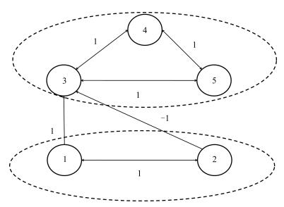
智能体间的拓扑关系如图 1所示, 机械臂的转角变化如图 2所示, 转动角速度变化如图 3所示.可以看出两组智能体在所设计的控制算法的作用下, 分别收敛于两个不同值, 实现了群一致性的要求.
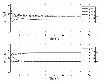 图 2 有向拓扑图下智能体位置状态信息Fig. 2 The position state of agents under the directed interaction graph
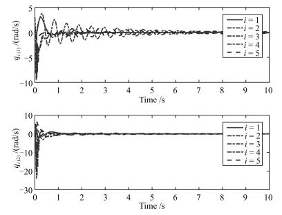 图 3 有向拓扑图下智能体速度信息Fig. 3 The velocities of agents under the directed interaction graph
4. 结论
本文主要研究了当系统拓扑结构为有向图时网络Euler-Lagrange系统的群一致性问题.在系统参数不确定时, 通过引入辅助变量构建状态方程, 设计了无需相对速度信息的分布式自适应控制律, 从而避免了实际中相对速度信息精度难以保证的情形.在所设计的控制律的控制作用下, 系统中每一组的智能体的状态信息均可以收敛于同一点, 而组与组之间的收敛点可以不同, 从而实现了群一致性.最后通过仿真验证了所提算法的有效性.
-
图 2 有向拓扑图下智能体位置状态信息
Fig. 2 The position state of agents under the directed interaction graph
-
[1] Oh K K, Park M C, Ahn H S. A survey of multi-agent formation control. Automatica, 2015, 53:424-440 doi: 10.1016/j.automatica.2014.10.022 [2] Su H S, Wang X F, Lin Z L. Flocking of multi-agents with a virtual leader. IEEE Transactions on Automatic Control, 2009, 54(2):293-307 doi: 10.1109/TAC.2008.2010897 [3] Yu H, Xia X H. Adaptive consensus of multi-agents in networks with jointly connected topologies. Automatica, 2012, 48(8):1783-1790 doi: 10.1016/j.automatica.2012.05.068 [4] Wu W, Zhou W J, Chen T P. Cluster synchronization of linearly coupled complex networks under pinning control. IEEE Transactions on Circuits and Systems I:Regular Papers, 2009, 56(4):829-839 doi: 10.1109/TCSI.2008.2003373 [5] Chen T P, Liu X W, Lu W L. Pinning complex networks by a single controller. IEEE Transactions on Circuits and Systems I:Regular Papers, 2007, 54(6):1317-1326 doi: 10.1109/TCSI.2007.895383 [6] Xu C J, Zheng Y, Su H S, Chen M Z Q, Zhang C F. Cluster consensus for second-order mobile multi-agent systems via distributed adaptive pinning control under directed topology. Nonlinear Dynamics, 2016, 83(4):1975-1985. doi: 10.1007/s11071-015-2459-5 [7] Xia W G, Cao M. Clustering in diffusively coupled networks. Automatica, 2011, 47(11):2395-2405 doi: 10.1016/j.automatica.2011.08.043 [8] Yu J Y, Wang L. Group consensus in multi-agent systems with switching topologies and communication delays. Systems and Control Letters, 2010, 59(6):340-348 doi: 10.1016/j.sysconle.2010.03.009 [9] Qin J H, Yu C B. Cluster consensus control of generic linear multi-agent systems under directed topology with acyclic partition. Automatica, 2013, 49(9):2898-2905 doi: 10.1016/j.automatica.2013.06.017 [10] Wen G G, Huang J, Wang C Y, Chen Z, Peng Z X. Group consensus control for heterogeneous multi-agent systems with fixed and switching topologies. International Journal of Control, 2016, 89(2):259-269 doi: 10.1080/00207179.2015.1072876 [11] 闵海波, 刘源, 王仕成, 孙富春.多个体协调控制问题综述.自动化学报, 2012, 38(10):1557-1570 http://www.aas.net.cn/CN/abstract/abstract17765.shtmlMin Hai-Bo, Liu Yuan, Wang Shi-Cheng, Sun Fu-Chun. An overview on coordination control problem of multi-agent system. Acta Automatica Sinica, 2012, 3810:1557-1570 http://www.aas.net.cn/CN/abstract/abstract17765.shtml [12] Cheng L, Hou Z G, Tan M. Decentralized adaptive consensus control for multi-manipulator system with uncertain dynamics. In:Proceedings of the 2008 IEEE International Conference on Systems, Man, and Cybernetics. Singapore:IEEE, 2008. 2712-2717 [13] Ren W. Distributed leaderless consensus algorithms for networked Euler-Lagrange systems. International Journal of Control, 2009, 82(11):2137-2149 doi: 10.1080/00207170902948027 [14] 梅杰, 张海博, 马广富.有向图中网络Euler-Lagrange系统的自适应协调跟踪.自动化学报, 2011, 37(5):596-603 http://www.aas.net.cn/CN/abstract/abstract17395.shtmlMei Jie, Zhang Hai-Bo, Ma Guang-Fu. Adaptive coordinated tracking for networked Euler-Lagrange systems under a directed graph. Acta Automatica Sinica, 2011, 375:596-603 http://www.aas.net.cn/CN/abstract/abstract17395.shtml [15] Mei J, Ren W, Ma G F. Distributed coordinated tracking with a dynamic leader for multiple Euler-Lagrange systems. IEEE Transactions on Automatic Control, 2011, 56(6):1415-1421 doi: 10.1109/TAC.2011.2109437 [16] Meng Z Y, Ren W, You Z. Distributed finite-time attitude containment control for multiple rigid bodies. Automatica, 2010, 46(12):2092-2099 doi: 10.1016/j.automatica.2010.09.005 [17] Mei J, Ren W, Ma G F. Distributed containment control for Lagrangian networks with parametric uncertainties under a directed graph. Automatica, 2012, 48(4):653-659 doi: 10.1016/j.automatica.2012.01.020 [18] Hu H X, Zhang Z, Yu L, Yu W W, Xie G M. Group consensus for multiple networked Euler-Lagrange systems with parametric uncertainties. Journal of Systems Science and Complexity, 2014, 27(4):632-649 doi: 10.1007/s11424-014-2149-2 [19] Liu J, Xiang L, Zhao L Y, Zhou J. Group consensus in uncertain networked Euler-Lagrange systems with acyclic interaction topology. In:Proceedings of the 34th Chinese Control Conference. Hangzhou, China:IEEE, 2015. 835-840 [20] Liu J, Ji J C, Zhou J, Xiang L, Zhao L Y. Adaptive group consensus in uncertain networked Euler-Lagrange systems under directed topology. Nonlinear Dynamics, 2015, 82(3):1145-1157 doi: 10.1007/s11071-015-2222-y [21] Mei J, Ren W, Chen J, Ma G F. Distributed adaptive coordination for multiple Lagrangian systems under a directed graph without using neighbors' velocity information. Automatica, 2013, 49(6):1723-1731 doi: 10.1016/j.automatica.2013.02.058 [22] Mei J, Ren W, Chen J. Distributed consensus of second-order multi-agent systems with heterogeneous unknown inertias and control gains under a directed graph. IEEE Transactions on Automatic Control, 2016, 61(8):2019-2034 doi: 10.1109/TAC.2015.2480336 [23] Spong M W, Hutchinson S, Vidyasagar M. Robot Modeling and Control. New Jersey, USA:John Wiley and Sons, 2006. [24] Mesbahi M, Egerstedt M. Graph Theoretic Methods in Multiagent Networks. New Jersey, USA:Princeton University Press, 2010. [25] Ren W, Beard R W. Distributed Consensus in Multi-Vehicle Cooperative Control. London, Britain:Springer-Verlag, 2008. [26] Yu W W, Chen G R, Gao M, Kurths J. Second-order consensus for multiagent systems with directed topologies and nonlinear dynamics. IEEE Transactions on Systems, Man, and Cybernetics, Part B (Cybernetics), 2010, 40(3):881-891 doi: 10.1109/TSMCB.2009.2031624 [27] Scardovi L, Arcak M, Sontag E D. Synchronization of interconnected systems with applications to biochemical networks:an input-output approach. IEEE Transactions on Automatic Control, 2010, 55(6):1367-1379 doi: 10.1109/TAC.2010.2041974 [28] Mei J. Weighted consensus for multiple Lagrangian systems under a directed graph. In:Proceedings of the 2015 Chinese Automation Congress (CAC). Wuhan, China:IEEE, 2015. 1064-1068 [29] Horn R A, Johnson C R. Matrix Analysis. New York, USA:Cambridge University Press, 1985. [30] Kelly R, Sáñtibanez V, Loría A. Control of Robot Manipulators in Joint Space. London, Britain:Springer, 2005. 期刊类型引用(7)
1. 孟祥正,吴爱国,梅杰,马广富. 有向图中含弹性关节多机械臂系统的分布式一致性. 中国科学:信息科学. 2023(01): 81-96 .  百度学术
百度学术2. 韩涛,关治洪,詹习生,严怀成,陈洁. 带有观测器的广义多智能体系统二分一致性. 控制理论与应用. 2023(01): 32-38 . 百度学术3. 杨盼,毕文豪,张安. 基于事件驱动的多智能体有限时间分群一致控制. 控制与决策. 2022(11): 2925-2933 . 百度学术4. 刘烨,杨朋举,张绪. 非线性多智能体磁滞系统的分布式输出反馈渐近一致控制. 控制理论与应用. 2021(07): 1102-1112 . 百度学术5. 王战红,李鹏程. 基于串空间的异构社交网络属性并行验证仿真. 计算机仿真. 2020(08): 409-413 . 百度学术6. 王卓,秦博东,徐雍,鲁仁全,魏庆来. 复杂无向网络连通性的一种高效判定算法. 自动化学报. 2020(10): 2129-2136 . 本站查看7. 曹然,程龙. 拒绝服务攻击下的Euler-Lagrange系统的安全控制. 空间控制技术与应用. 2018(05): 76-80+88 . 百度学术其他类型引用(7)
-

 下载:
下载:
 下载:
下载:
计量
- 文章访问数: 2595
- HTML全文浏览量: 294
- PDF下载量: 669
- 被引次数: 14
