

-
摘要: 针对具有执行器故障和未知扰动的线性广义系统,提出一种新的故障估计器设计方法.所设计的故障估计器具有非奇异结构,便于实现.在故障频域范围有限的条件下,为了抑制未知扰动和有限频域故障对故障估计误差的影响,基于广义Kalman-Yakubovich-Popov(KYP)引理给出了故障估计器的鲁棒性设计条件,并将其转化为方便求解的线性矩阵不等式形式.最后,通过一个电路系统的仿真算例验证了所提出方法的有效性.
-
关键词:
- 广义系统 /
- 故障估计器 /
- 广义Kalman-Yakubovich-Popov (KYP)引理 /
- 有限频域
Abstract: This paper proposes a novel fault estimator design method for linear descriptor systems with actuator fault and unknown disturbance. The proposed fault estimator has a nonsingular structure and hence is easy to implement. Under the condition that faults belong to a finite frequency domain, the generalized Kalman-Yakubovich-Popov (KYP) lemma is used to propose robust design conditions to attenuate the effect of unknown disturbance and faults on the fault estimation error. Moreover, the design conditions are converted to linear matrix inequalities, which can be solved easily. Finally, an electrical circuit is simulated to verify the effectiveness of the proposed method. -
故障诊断技术为提高系统安全性和可靠性提供了一条有效的途径, 在过去的几十年里得到了国内外学者的广泛关注.故障诊断的主要任务可以分为故障检测、故障分离和故障估计.由于故障的幅值信息是后续容错处理的重要基础, 近年来, 故障估计问题得到了一定的重视, 文献中出现了自适应故障诊断观测器[1-2]、滑模故障估计[3]、基于状态增广的故障估计[4]等诸多故障估计方法.另一方面, 考虑到广义系统比常见的状态空间系统更具有一般性, 一些学者们对广义系统的故障诊断问题展开了研究[5-9].在广义系统的故障估计方面, 文献[5]提出了基于高增益观测器的故障估计方法, 文献[7]利用比例积分观测器进行故障估计, 文献[8]和文献[9]分别提出了自适应神经网络观测器和自适应观测器, 用于广义系统的故障估计.
近年来, 有些学者考虑到故障通常处于有限频域范围内, 并利用这一特点研究了一系列有限频域故障诊断方法[10-14].由于有限频域设计能够有效降低故障诊断算法的设计保守性, 该设计思想在Takagi-Sugeno (T-S)模糊系统、网络控制系统等复杂系统的故障诊断中得到了进一步的推广应用与深入研究[15-17].文献[18]针对线性时滞系统提出了一种基于状态观测器的故障估计器, 文献[19]进一步研究了故障处于有限频域范围时的故障估计与容错处理问题.与一些其他故障估计方法(例如高增益观测器[5]、自适应神经网络观测器[8])相比, 这种方法的优点是结构更加简单且运算量更小.但是文献[19]只研究了常规状态空间系统的情况.虽然有限频域故障诊断方法在常义系统中得到了深入研究, 但是在广义系统的有限频域故障估计方面的研究还非常少见, 目前只有文献[20]利用有限频域设计法研究了广义系统的故障估计问题, 但是文献[20]研究的是存在有限频域扰动时的故障估计问题, 并且需要假设故障的高阶导数为零.受文献[19]的启发, 本文将基于观测器的故障估计器设计思想推广到广义系统, 提出了一种非奇异形式的故障估计器, 并基于广义Kalman-Yakubovich-Popov (KYP)引理推导了一种新的鲁棒性设计条件, 以抑制故障和扰动对故障估计误差的影响.需要指出的是, 本文研究的是故障处于有限频域范围内时的故障估计方法, 对故障的具体动态并无要求, 也不要求扰动处于有限频域范围内.
1. 问题描述
考虑如下描述系统
$ \begin{cases} E\dot{{\pmb x}}(t) = A{\pmb x}(t) + B{\pmb u}(t) +B_d{\pmb d}(t) +B_f {\pmb f}(t) \\ {\pmb y}(t) = C{\pmb x}(t) + D_{d}{\pmb d}(t) \end{cases} $
(1) 其中, ${\pmb x}(t)\in {\boldsymbol{\rm{R}}}^{n}$, ${\pmb u}(t)\in{\boldsymbol{\rm{R}}}^{p}$, ${\pmb y}(t)\in{\boldsymbol{\rm{R}}}^{m}$分别是状态向量、控制输入和测量输出, ${\pmb d}(t)\in{\boldsymbol{\rm{R}}}^{l}$是未知扰动, ${\pmb f}(t)\in{\bf R}^{q}$表示执行器故障. $E$, $A$, $B$, $B_d$, $B_f$, $C$, $D_d$是具有适当维数的常值矩阵, 其中矩阵$E$可能是奇异的, 即${\rm{rank}} (E) \leq n$.不失一般性, 本文假设矩阵$E$和$C$满足如下条件
$ {\rm{rank}} \left[ \begin{matrix} E \\ C \end{matrix} \right] = n $
(2) 另外, 假设故障的频率范围是已知的, 即
$ \vert \omega \vert \leq \varpi $
(3) 这表明故障处于低频范围内.
注1.需要说明的是, 系统(1)中的$d(t)$集成了系统中的不确定性, 它可以是既包含过程扰动又包含测量噪声的.例如, 如果所考虑的系统本来具有如下形式
$ \begin{cases} E\dot{{\pmb x}}(t) = A{\pmb x}(t) +B{\pmb u}(t)+B_w {\pmb w}(t)+B_f {\pmb f}(t)\\ {\pmb y}(t) = C{\pmb x}(t)+D_v{\pmb v}(t) +D_f {\pmb f}(t) \end{cases} $
(4) 则可通过令
$ {\pmb d}(t) = \left[\begin{matrix} {\pmb w}(t) \\ {\pmb v}(t) \end{matrix} \right] $
(5) 将其写成式(1)的形式, 其中
$ B_d = \left[\begin{matrix} B_w & 0 \end{matrix} \right], \quad D_d = \left[\begin{matrix} 0 & D_v \end{matrix} \right] $
(6) 对于系统(1), 提出如下形式的故障估计器
$ \begin{cases} \dot{{\pmb z}}(t) = TA\hat{{\pmb x}}(t) + TB{\pmb u}(t) +L({\pmb y}(t)-C\hat{{\pmb x}}(t)) \\ \hat{{\pmb x}}(t) = {\pmb z}(t) + {N{\pmb y}(t)} \\ \hat{{\pmb f}}(t) =V({\pmb y}(t)-C\hat{{\pmb x}}(t)) \end{cases} $
(7) 其中, ${\pmb z}(t)\in{\boldsymbol{\rm{R}}}^{n}$是故障估计器的状态变量, $\hat{{\pmb x}}(t)\in{\boldsymbol{\rm{R}}}^{n}$是状态估计向量, $\hat{{\pmb f}}(t)\in{\bf R}^{q}$是执行器故障估计向量. $T\in{\boldsymbol{\rm{R}}}^{n\times n }$, $N$ $\in$ ${\boldsymbol{\rm{R}}}^{n\times m}$, $L \in{\boldsymbol{\rm{R}}}^{n\times m }$, $V \in{\boldsymbol{\rm{R}}}^{q \times m}$是待设计的参数矩阵, 其中, 矩阵$T$和$N$需要满足如下条件
$ TE+NC=I_n $
(8) 其中, $I_n$表示$n\times n$维的单位矩阵.
本文的目标是使故障估计尽可能地近似真实故障.为了分析故障估计的准确程度, 定义状态估计误差${\pmb e}(t)$和故障估计误差$\tilde{{\pmb f}}(t)$如下
$ {\pmb e}(t) = {\pmb x}(t) - \hat{{\pmb x}}(t) $
(9) $ \tilde{{\pmb f}}(t) = {\pmb f}(t) - \hat{{\pmb f}}(t) $
(10) 由式(1), 式(7)和式(8)可得
$ \dot{{\pmb e}}(t) = \dot{{\pmb x}}(t) - \dot{\hat{{\pmb x}}}(t)= \\ TA{\pmb x}(t) +TB{\pmb u}(t) +TB_d{\pmb d}(t) +TB_f {\pmb f}(t) +\\ NC\dot{{\pmb x}}(t) - TA\hat{{\pmb x}}(t)-TB{\pmb u}(t) -\\ L({\pmb y}(t)-C\hat{{\pmb x}}(t))-N\dot{{\pmb y}}(t) =\\ (TA-LC){\pmb e}(t)+TB_f{\pmb f}(t) + \\ (TB_d -LD_d){\pmb d}(t) -ND_d \dot{{\pmb d}}(t) $
(11) 另外, 将$\hat{{\pmb f}}(t) = V({\pmb y}(t)-C\hat{{\pmb x}}(t))$代入式(10)可得
$ \tilde{{\pmb f}}(t) = {\pmb f}(t) -VC{\pmb e}(t)-VD_d{\pmb d}(t) $
(12) 根据式(11)和式(12), 可以得到如下的误差系统
$ \begin{cases} \dot{{\pmb e}}(t) = (TA-LC){\pmb e}(t)+TB_f{\pmb f}(t) +\\ \qquad\ \ (TB_d-LD_d) {\pmb d}(t) -ND_d \dot{{\pmb d}}(t)\\ \tilde{{\pmb f}}(t) = {\pmb f}(t) - VC{\pmb e}(t)-VD_d{\pmb d}(t) \end{cases} $
(13) 令$\bar{{\pmb d}}(t) = \bigl[{matrix} {\pmb d}^{\rm T}(t)&\dot{{\pmb d}}^{\rm T}(t) {matrix} \bigr] ^{\rm T}$, 可将误差系统(13)表示成如下形式
$ \begin{cases} \dot{{\pmb e}}(t) = (TA-LC){\pmb e}(t)+TB_f{\pmb f}(t) +\tilde{B}_d\bar{{\pmb d}}(t) \\ \tilde{{\pmb f}}(t) = -VC{\pmb e}(t) + {\pmb f}(t) +\tilde{D}_d \bar{{\pmb d}}(t) \end{cases} $
(14) 其中, $\tilde{B}_d = [{matrix} TB_d-LD_d \;\;\;-ND_d {matrix}]$, $ \tilde{D}_d = [{matrix}-VD_d \;\;\; 0 {matrix}] $.
现在我们可以将故障估计器的设计问题描述为设计矩阵$T$, $N$, $L$和$V$(其中$T$和$N$满足条件(8))使得误差系统(14)稳定, 且满足如下性能指标
$ \Vert G_{\tilde{{f}}{ f}}(s) \Vert^{[-\varpi, \varpi]}_{\infty} < \gamma_f $
(15) $ \Vert G_{\tilde{{ f}}\bar{{ d}}}(s) \Vert_{\infty} < \gamma_d $
(16) 其中, $G_{\tilde{{ f}}{ f}}(s)$和$G_{\tilde{{ f}}\bar{{ d}}}(s)$分别是从${\pmb f}(t)$到$\tilde{{\pmb f}}(t)$的传递函数和从$\bar{{\pmb d}}(t)$到$\tilde{{\pmb f}}(t)$的传递函数.
2. 故障估计器设计
本节介绍故障估计器(7)的设计方法.首先, 设计$T$和$N$使之满足等式约束(8).由文献[21]可知, 满足式(8)的$T$和$N$可由下式确定
$ \begin{cases} T = \Theta^{\dagger} {\alpha_T} + S(I_{n+m} -\Theta \Theta^{\dagger}) {\alpha_T} \\ N = \Theta^{\dagger} {\alpha_N} + S(I_{n+m} -\Theta \Theta^{\dagger}) {\alpha_N} \end{cases} $
(17) 其中, $S\in{\boldsymbol{\rm{R}}}^{n\times (n+m)}$是可以任意选取的矩阵, 矩阵$\Theta \in {\boldsymbol{\rm{R}}}^{(n+m)\times n}$, $ \alpha_{T}\in {\boldsymbol{\rm{R}}}^{(n+m)\times n}$, $ \alpha_{N} \in {\boldsymbol{\rm{R}}}^{(n+m)\times m}$为
$ \Theta = \left[ \begin{matrix} E \\ C \end{matrix} \right], \ \ {\alpha_T} = \bigl[\begin{matrix} I_n & 0 \end{matrix}\bigr], \ \ {\alpha_N} = \bigl[\begin{matrix} 0 & I_m \end{matrix}\bigr] $
得到满足式(8)的$T$和$N$之后, 可以基于误差系统(14)分析故障估计器(7)满足稳定性及性能指标(15)和(16)要求的条件.
在给出本文的主要结果之前, 先给出下面的有用引理.
引理1(广义KYP引理) [22].对于传递函数$G(s)=$ $\mathcal{C}(sI-\mathcal{A})^{-1}\mathcal{B}+\mathcal{D}$和给定一个对称矩阵$\Pi$, 下面的两个条件是等价的:
1) 下面的有限频域不等式成立
$ \left[\begin{matrix} G({\rm j}\omega) \\ I \end{matrix} \right] ^{\rm T} \Pi \left[\begin{matrix} G({\rm j}\omega) \\ I \end{matrix} \right] <0, \ \forall \omega \in \Omega $
(18) 其中, $\Omega$由表 1给出.
表 1 不同频率范围的$\Omega$和$\Xi$Table 1 $\Omega$ and $\Xi$ corresponding to different frequency ranges低频范围 中频范围 高频范围 $\Omega$ $\vert \omega \vert \leq \varpi _l$ $\varpi_1\leq \omega \leq \varpi_2 $ $\vert \omega \vert \geq \varpi _h$ $\Xi$ $\left[ {matrix} -\mathcal{Q} & \mathcal{P} \\ \mathcal{P} & \varpi^2_l \mathcal{Q} {matrix} \right] $ $\left[ {matrix} -\mathcal{Q} & \mathcal{P}+j\varpi _c \mathcal{Q} \\ \mathcal{P} -j\varpi _c \mathcal{Q} & -\varpi_1\varpi_2 \mathcal{Q} {matrix} \right] $ $\left[ {matrix} \mathcal{Q} & \mathcal{P} \\ \mathcal{P} & -\varpi^2_h \mathcal{Q} {matrix} \right] $ 2) 存在共轭对称矩阵$\mathcal{P}$和$\mathcal{Q}$, $\mathcal{Q}>0$满足
$ \left[\begin{matrix} \mathcal{A} & \mathcal{ B} \\ I & 0 \end{matrix} \right] ^{\rm T} \Xi \left[\begin{matrix} \mathcal{A} & \mathcal{B} \\ I & 0 \end{matrix} \right] + \left[\begin{matrix} \mathcal{C} & \mathcal{D} \\ 0 & I \end{matrix} \right] ^{\rm T} \Pi \left[\begin{matrix} \mathcal{C} & \mathcal{ D} \\ 0 & I \end{matrix} \right] <0 $
(19) 其中, $\Xi$由表 1给出, 且$\varpi _c = (\varpi_1 +\varpi_2)/2$.
引理2 (Finsler引理)[23].对于$\mathscr{Q} \in{\boldsymbol{\rm{R}}}^{ {a \times a}}$, $\mathscr{U} \in{\boldsymbol{\rm{R}}}^{ {a \times b}}$, 下面的两个条件是等价的:
1) 矩阵不等式
$ \mathscr{U} ^{\perp} \mathscr{Q} (\mathscr{U}^{\perp})^{\rm T} <0 $
成立, 其中$\mathscr{U}^{\perp}$是任意满足$\mathscr{U} ^{\perp} \mathscr{U} =0$的矩阵.
2) 存在一个矩阵$ \mathscr{Y} \in{\boldsymbol{\rm{R}}}^{ {b \times a}} $, 使得
$ \mathscr{Q}+ \mathscr{U} \mathscr{Y}+\mathscr{Y}^{\rm T} \mathscr{U}^{\rm T} <0 $
引理3[24].连续状态空间系统
$ \begin{cases} \dot{{\pmb x}}(t) = \mathcal{A}{\pmb x}(t)+\mathcal{B}{\pmb w}(t)\\ {\pmb y}(t) = \mathcal{C} {\pmb x}(t) + \mathcal{D} {\pmb w}(t) \end{cases} $
(20) 是稳定的, 并且其传递函数
$ G(s) =\mathcal{C} (sI- \mathcal{A})^{-1}\mathcal{B} + \mathcal{D} $
(21) 满足$\Vert G(s) \Vert _{\infty} < \gamma$的充分必要条件是存在一个对称矩阵$\mathcal{P}$ $>$ $0$, 使得如下矩阵不等式成立
$ \left[\begin{matrix} \mathcal{A}^{\rm T}\mathcal{P} + \mathcal{P} \mathcal{A} + \mathcal{C}^{\rm T}\mathcal{C} & \mathcal{P} \mathcal{B} +\mathcal{C}^{\rm T}\mathcal{D} \\ \mathcal{B}^{\rm T} \mathcal{P} +\mathcal{D}^{\rm T}\mathcal{C } & \mathcal{D}^{\rm T}\mathcal{D}-\gamma^2I \end{matrix} \right] <0 $
(22) 引理1是广义KYP引理, 它是有限频域设计的重要基础.引理3则是著名的有界实引理, 是全频域$H_{\infty}$分析与设计的重要工具.若令$\mathcal{Q} = 0$, $\Pi = \mathit{\boldsymbol{diag}}\left\{I, -\gamma^2 I \right\}$, $\mathcal{P}>0$, 则广义KYP引理退化为有界实引理.所以, 有界实引理是广义KYP引理在全频域条件下的特殊形式.
为了保证性能指标(15), 本文基于引理1和引理2给出如下定理.
定理1.对于传递函数$G(s)=\mathcal{C}(sI-\mathcal{A})^{-1}\mathcal{B}+\mathcal{D}$和一个给定的对称矩阵$\Pi$, 我们有如下结果:
1) $G(s)$满足如下有限频域不等式
$ \left[\begin{matrix} G({\rm j}\omega) \\ I \end{matrix} \right] ^{\rm T} \Pi \left[\begin{matrix} G({\rm j}\omega) \\ I \end{matrix} \right] <0, \ \ \forall \vert \omega \vert \leq \varpi_l $
(23) 的充分必要条件是存在共轭对称矩阵$\mathcal{P}$和$\mathcal{Q}$, $\mathcal{Q}>0$以及具有适当维数的矩阵$\mathcal{M}_1$, $\mathcal{M}_2$, $\mathcal{G}$, 使得如下矩阵不等式成立
$ \left[\begin{matrix} \Theta_l + \bar{\mathcal{M}}\bar{\mathcal{A}} +\bar{\mathcal{A}}^{\rm T}\bar{\mathcal{M}}^{\rm T}& * \\ -\bar{\mathcal{M}}^{\rm T} +\bar{\mathcal{P}}_l^{\rm T} +\mathcal{G} \bar{\mathcal{A}} & -\mathcal{Q}-\mathcal{G}-\mathcal{G}^{\rm T} \end{matrix} \right] <0 $
(24) 其中
$ \bar{\mathcal{M}} = \left[\begin{matrix} \mathcal{M}_1 \\ \mathcal{M}_2 \end{matrix} \right], \ \bar{\mathcal{A}} = \left[\begin{matrix} \mathcal{A} & \mathcal{B} \end{matrix} \right], \ \bar{\mathcal{P}}_l = \left[\begin{matrix} \mathcal{P} \\ 0 \end{matrix} \right] \\ \Theta_l = \left[\begin{matrix} \varpi^2_l\mathcal{Q} & 0 \\ 0 & 0 \end{matrix} \right] + \left[\begin{matrix} \mathcal{C} & \mathcal{D} \\ 0 & I \end{matrix} \right] ^{\rm T} \Pi \left[\begin{matrix} \mathcal{C} & \mathcal{ D} \\ 0 & I \end{matrix} \right] $
2) $G(s)$满足如下有限频域不等式
$ \left[\begin{matrix} G({\rm j}\omega) \\ I \end{matrix} \right] ^{\rm T} \Pi \left[\begin{matrix} G({\rm j}\omega) \\ I \end{matrix} \right] <0, \ \ \forall \varpi_1 \leq \omega \leq \varpi_2 $
(25) 的充分必要条件是存在共轭对称矩阵$\mathcal{P}$和$\mathcal{Q}$, $\mathcal{Q}>0$以及具有适当维数的矩阵$\mathcal{M}_1$, $\mathcal{M}_2$, $\mathcal{G}$, 使得如下矩阵不等式成立
$ \left[\begin{matrix} \Theta_l + \bar{\mathcal{M}}\bar{\mathcal{A}} +\bar{\mathcal{A}}^{\rm T}\bar{\mathcal{M}}^{\rm T} & * \\ -\bar{\mathcal{M}}^{\rm T} +\bar{\mathcal{P}}_l^{\rm T} +\mathcal{G} \bar{\mathcal{A}} & -\mathcal{Q}-\mathcal{G}-\mathcal{G}^{\rm T} \end{matrix} \right] <0 $
(26) 其中, $\bar{\mathcal{M}}$和$\bar{\mathcal{A}}$的定义由式(25)给出, 矩阵$\Theta _m$和$\bar{\mathcal{P}}_m$的形式分别为
$ \Theta_m = \left[\begin{matrix} -\varpi_1 \varpi_2 \mathcal{Q} & 0 \\ 0 & 0 \end{matrix} \right] + \left[\begin{matrix} \mathcal{C} & \mathcal{D} \\ 0 & I \end{matrix} \right] ^{\rm T} \Pi \left[\begin{matrix} \mathcal{C} & \mathcal{ D} \\ 0 & I \end{matrix} \right] \\ \bar{\mathcal{P}}_m = \left[\begin{matrix} \mathcal{P}-{\rm j} \varpi _c \mathcal{Q} \\ 0 \end{matrix} \right] $
(27) 3) $G(s)$满足有限频域不等式
$ \left[\begin{matrix} G({\rm j}\omega) \\ I \end{matrix} \right] ^{\rm T} \Pi \left[\begin{matrix} G({\rm j}\omega) \\ I \end{matrix} \right] <0, \ \ \forall \vert \omega \vert \geq \varpi_h $
(29) 的充分必要条件是存在具有适当维数的共轭对称矩阵$\mathcal{P}$和$\mathcal{Q}$, $\mathcal{Q}>0$以及矩阵$\mathcal{M}_1$, $\mathcal{M}_2$, $\mathcal{G}$, 使得
$ \left[\begin{matrix} \Theta_h + \bar{\mathcal{M}}\bar{\mathcal{A}} +\bar{\mathcal{A}}^{\rm T}\bar{\mathcal{M}}^{\rm T} & * \\ -\bar{\mathcal{M}}^{\rm T} +\bar{\mathcal{P}}_h^{\rm T} +\mathcal{G}\bar{\mathcal{A}} & \mathcal{Q}-\mathcal{G}-\mathcal{G}^{\rm T} \end{matrix} \right] <0 $
(30) 其中, $\bar{\mathcal{M}}$和$\bar{\mathcal{A}}$的定义由式(25)给出, 矩阵$\Theta _h$和$\bar{\mathcal{P}}_h$的形式为
$ \Theta_h = \left[\begin{matrix} -\varpi^2_h \mathcal{Q} & 0 \\ 0 & 0 \end{matrix} \right] + \left[\begin{matrix} \mathcal{C} & \mathcal{D} \\ 0 & I \end{matrix} \right] ^{\rm T} \Pi \left[\begin{matrix} \mathcal{C} & \mathcal{ D} \\ 0 & I \end{matrix} \right], \ \bar{\mathcal{P}}_h = \left[\begin{matrix} \mathcal{P} \\ 0 \end{matrix} \right] $
(31) 证明.根据引理1, 频域不等式(18)在低频范围内成立等价于
$ \left[\begin{matrix} \mathcal{A} & \mathcal{ B} \\ I & 0 \end{matrix} \right] ^{\rm T} \left[\begin{matrix}-\mathcal{Q} & \mathcal{P} \\ \mathcal{P} & \varpi^2_l \mathcal{Q} \end{matrix} \right] \left[\begin{matrix} \mathcal{A} & \mathcal{B} \\ I & 0 \end{matrix} \right] +\\ \left[\begin{matrix} \mathcal{C} & \mathcal{D} \\ 0 & I \end{matrix} \right] ^{\rm T} \Pi \left[\begin{matrix} \mathcal{C} & \mathcal{ D} \\ 0 & I \end{matrix} \right] <0 $
(32) 易知式(32)可以写成如下形式
$ \left[\begin{matrix} I & \bar{\mathcal{A} } ^{\rm T} \end{matrix} \right] \left[\begin{matrix} \Theta_l & \bar{\mathcal{P}}_l \\ \bar{\mathcal{P}}^{\rm T}_l &-\mathcal{Q} \end{matrix} \right] \left[\begin{matrix} I \\ \bar{\mathcal{A} } \end{matrix} \right] <0 $
(33) 取
$ \mathscr{U} = \left[\begin{matrix} \bar{\mathcal{A}}^{\rm T} \\ -I \end{matrix} \right] $
(34) 则有
$ \mathscr{U}^{\perp} = \left[\begin{matrix} I & \bar{\mathcal{A}}^{\rm T} \end{matrix} \right] $
此时, 矩阵不等式(33)可以表示为
$ \mathscr{U}^{\perp} \left[\begin{matrix} \Theta_l & \bar{\mathcal{P}}_l \\ \bar{\mathcal{P}}^{\rm T}_l &-\mathcal{Q} \end{matrix} \right] (\mathscr{U}^{\perp})^{\rm T} <0 $
(35) 根据引理2, 式(35)成立的充分必要条件是存在一个矩阵$\mathscr{Y} $, 使得
$ \left[\begin{matrix} \Theta_l & \bar{\mathcal{P}}_l \\ \bar{\mathcal{P}}^{\rm T}_l &-\mathcal{Q} \end{matrix} \right] + \mathscr{U} \mathscr{Y} + \mathscr{Y} ^{\rm T} \mathscr{U}^{\rm T} <0 $
(36) 成立.
令
$ \mathscr{Y} = \left[\begin{matrix} \mathcal{M}_1^{\rm T} & \mathcal{M}_2^{\rm T} & \mathcal{G}^{\rm T} \end{matrix} \right] $
(37) 并将式(34)和式(37)代入式(36), 即可得到式(24).
利用相同的原理, 可以证明中频范围和高频范围内的结论.此处从略.
注2.定理1基于广义Kalman-Yakubovich-Popov引理和Finsler引理, 给出了广义KYP引理的一种等价形式, 为有限频域设计过程中的参数选取提供了更方便、更直观的条件.这一结果不仅可以用于故障诊断观测器设计, 也可用于其他有限频域设计, 例如有限频域$H_{\infty}$滤波和有限频域鲁棒控制器设计.因此, 定理1是本文的主要贡献之一.
基于定理1, 我们提出下面的定理, 用于设计故障估计器使其满足性能指标(15).
定理2.给定$\gamma_f > 0 $, 故障估计器(7)使得误差系统(14)满足有限频域性能指标(15)的充分条件是存在对称矩阵$P_{1}\in{\bf R}^{n \times n}$, $Q \in{\boldsymbol{\rm{R}}}^{n \times n}$, $Q>0$, 以及矩阵$G\in{\boldsymbol{\rm{R}}}^{n\times n}$, $V$ $\in$ ${\boldsymbol{\rm{R}}}^{q\times m}$, $L\in{\boldsymbol{\rm{R}}}^{n\times m}$, 使得矩阵不等式(38)成立.
$ \left[\begin{matrix} \tilde{\Phi}_{11} & * & * & * \\ \tilde{\Phi}_{21} & \tilde{\Phi}_{22} & * & * \\ \tilde{\Phi}_{31} &\tilde{\Phi}_{32} & \tilde{\Phi}_{33} & * \\ -VC & I_q & 0 &-I_q \end{matrix} \right] <0 $
(38) 其中,
$ \tilde{\Phi}_{11} = \varpi^2 Q +{\rm{He}}\left\{ \alpha_1 G(T A-L C) \right\} \\ \tilde{\Phi}_{21} = \alpha_1 (TB_f)^{\rm T}G^{\rm T} + V_1^{\rm T}G(TA-LC) \\ \tilde{\Phi}_{22}= -\gamma_f^2 I_q + {\rm{He}}\left\{V_1^{\rm T}G TB_f \right\} \\ \tilde{\Phi}_{31} = -\alpha_1G^{\rm T}+ G( TA-LC) + P_{1} \\ \tilde{\Phi}_{32}= -G^{\rm T} V_1+ GTB_f \\ \tilde{\Phi}_{33}= -Q-G-G^{\rm T} $
这里的$\alpha_1 \in{\boldsymbol{\rm{R}}}$和$V_1 \in{\boldsymbol{\rm{R}}} ^{n\times q} $是事先确定的设计参数.在本文中, 为了形式更加紧凑, 我们用$*$表示矩阵中可由对称性得到的项, 用${\rm{He}}\left\{ M \right\}$表示$M+M^{\rm T}$.
证明.若将式(18)中的$\Pi$取为
$ \Pi =\left[ \begin{matrix} I_q & 0 \\ 0 &-\gamma_f^2 I_q \end{matrix} \right] $
则有限频域不等式(18)即可成为式(15).由定理1可知, 式(18)成立的充分必要条件是存在对称矩阵$\mathcal{P}$, $\mathcal{Q}>0$和矩阵$\mathcal{M}_1$, $\mathcal{M}_2$, $\mathcal{G}$, 使得不等式(39)成立.
$ \left[\begin{matrix} \varpi^2 \mathcal{Q} +\mathcal{C}^{\rm T}\mathcal{C} +{\rm{He}} \left\{ \mathcal{M}_1\mathcal{A} \right\} & * \\ \mathcal{M}_2\mathcal{A}+ \mathcal{B}^{\rm T}\mathcal{M}^{\rm T}_1 + \mathcal{D}^{\rm T}\mathcal{C} & {\rm{He}}\left\{ \mathcal{M}_2\mathcal{B} \right\} +\mathcal{D}^{\rm T}\mathcal{D}-\gamma_f^2I_q \\ -\mathcal{M}^{\rm T}_1 + \mathcal{P} +\mathcal{G} \mathcal{A} &- \mathcal{M}^{\rm T}_2 +\mathcal{G} \mathcal{B} \end{matrix} \right. \\ \left.\begin{matrix} & * \\ & * \\ & -\mathcal{Q}-\mathcal{G}-\mathcal{G}^{\rm T} \end{matrix} \right] <0 $
(39) 令
$ \mathcal{A} = TA- LC, \ \mathcal{B} = TB_f, \ \mathcal{C} =-VC , \ \mathcal{D} = I_q \\ \mathcal{Q}=Q, \ \mathcal{P} =P_1, \ \mathcal{M}_1 =\alpha_1G, \ \mathcal{M}_2 = V_1^{\rm T} G, \ \mathcal{G}=G $
并将$\mathcal{A}$, $\mathcal{B}$, $\mathcal{C}$, $\mathcal{D}$, $\mathcal{Q}$, $\mathcal{P}$, $\mathcal{M}_1$, $\mathcal{M}_2$, $\mathcal{G}$代入条件(39)中可得
$ \left[\begin{matrix} \Phi_{11} & * & * \\ \Phi_{21} & \Phi_{22} & * \\ \Phi_{31} & \Phi_{32} & \Phi_{33} \end{matrix} \right] <0 $
(40) 其中,
$ \Phi_{11} = \varpi^2 Q +(VC)^{\rm T}VC +{\rm{He}}\left\{ \alpha_1 G(T A -LC) \right\} \\ \Phi_{21} = \alpha_1 TB_f^{\rm T}G^{\rm T} + V_1^{\rm T}G(TA-LC) \\ \Phi_{22} = -\gamma_f^2 I_q + V_1^{\rm T}G TB_f + (TB_f)^{\rm T}G^{\rm T} V_1 \\ \Phi_{31} = -\alpha_1G^{\rm T}+ G( TA-LC) +P_{1} \\ \Phi_{32} = -G^{\rm T} V_1+ GTB_f\\ \Phi_{33} = - Q-G -G^{\rm T} $
然后, 利用Schur补引理[25]可得式(40)等价于式(38).
综上, 如果式(38)成立, 则误差系统(14)满足有限频域性能指标(15).
下面的定理基于有界实引理给出误差系统(14)稳定, 且满足性能指标(16)的条件.
定理3.给定$\gamma_d> 0 $, 故障估计器(7)使得误差系统(14)稳定且满足有限频域性能指标(16)的充分条件是存在对称矩阵$P_{2}\in{\bf R}^{n \times n}$和矩阵$G\in{\boldsymbol{\rm{R}}}^{n\times n}$, $V\in{\bf R}^{q\times m}$, $L$ $\in$ ${\boldsymbol{\rm{R}}}^{n\times m}$, 使得矩阵不等式(41)成立.
$ \left[\begin{matrix} \tilde{\Psi}_{11} & * & * & * & * \\ \tilde{\Psi}_{21} &-\gamma_d^2 I_l & * & * & * \\ \tilde{\Psi}_{31} & 0 &-\gamma_d^2 I_l & * & * \\ \tilde{\Psi}_{41} & \tilde{\Psi}_{42} &-GND_d & \tilde{\Psi}_{44} & * \\ -VC & -VD_d & 0 & 0 & -I_q \end{matrix} \right] <0 $
(41) 其中,
$ \tilde{\Psi}_{11} = {\rm{He}}\left\{ \alpha_2 G(T A-L C) \right\} \\ \tilde{\Psi}_{21} = \alpha_2 (TB_d-LD_d)^{\rm T}G^{\rm T} \\ \tilde{\Psi}_{31} = -\alpha_2 (ND_d)^{\rm T}G^{\rm T} \\ \tilde{\Psi}_{41} = -\alpha_2 G^{\rm T}+ G( TA-LC) + P_{2} \\ \tilde{\Psi}_{42} = G(TB_d-LD_d)\\ \tilde{\Psi}_{44} = -G-G^{\rm T} $
这里$\alpha_2 \in{\boldsymbol{\rm{R}}}$是事先确定的设计参数.
证明.在引理1中, 令
$ \mathcal{Q} = 0, \quad \Pi =\left[ \begin{matrix} I_q & 0 \\ 0 &-\gamma_d^2 I_l \end{matrix} \right] $
则可得到引理3中的矩阵不等式(22).因此, 我们也可以利用定理1将矩阵不等式(22)转化为不等式(42)形式.
$ \left[\begin{matrix} \mathcal{C}^{\rm T}\mathcal{C} +{\rm{He}}\left\{ \mathcal{M}_1\mathcal{A} \right\} & * \\ \mathcal{M}_2\mathcal{A}+ \mathcal{B}^{\rm T}\mathcal{M}^{\rm T}_1 + \mathcal{D}^{\rm T} \mathcal{C} & {\rm{He}}\left\{ \mathcal{M}_2\mathcal{B} \right\} +\mathcal{D}^{\rm T} \mathcal{D}-\gamma_d^2I_l \\ -\mathcal{M}^{\rm T}_1 + \mathcal{P} +\mathcal{G} \mathcal{A} &- \mathcal{M}^{\rm T}_2 +\mathcal{G} \mathcal{B} \end{matrix} \right. \\ \left.\begin{matrix}& * \\& * \\&-\mathcal{G}-\mathcal{G}^{\rm T}\end{matrix} \right] <0 $
(42) 令
$ \mathcal{A} = TA- LC, \ \mathcal{B} = \tilde{B}_d, \ \mathcal{C} =-VC, \ \mathcal{D} =\tilde{D}_d \\ \mathcal{P} =P_2, \ \mathcal{M}_1 =\alpha_2G, \ \mathcal{M}_2 = 0, \ \mathcal{G}=G $
并利用Schur补引理可知由式(41)可以推出式(22).因此, 如果式(41)成立, 则误差系统(14)稳定且满足性能指标(16).
基于定理2和定理3的结果, 下面的定理给出了故障估计器的设计方法.
定理4.对于给定的$\gamma_f > 0 $和$\gamma_d>0$, 如果存在对称矩阵$P_{1}$, $P_{2}$, $Q \in{\boldsymbol{\rm{R}}}^{n \times n}$, $Q>0$, 以及矩阵$G\in{\boldsymbol{\rm{R}}}^{n\times n}$, $V$ $\in$ ${\bf R}^{q\times m}$, $W\in{\boldsymbol{\rm{R}}}^{n\times m}$, 使得如下线性矩阵不等式成立
$ \left[\begin{matrix} \tilde{\Phi}'_{11} & * & * & * \\ \tilde{\Phi}'_{21} & \tilde{\Phi}'_{22} & * & * \\ \tilde{\Phi}'_{31} &\tilde{\Phi}'_{32} & \tilde{\Phi}'_{33} & * \\ -VC & I_q & 0 &-I_q \end{matrix} \right] <0 $
(43) $ \left[\begin{matrix} \tilde{\Psi}'_{11} & * & * & * & * \\ \tilde{\Psi}'_{21} &-\gamma_d^2 I_l & * & * & * \\ \tilde{\Psi}'_{31} & 0 &-\gamma_d^2 I_l & * & * \\ \tilde{\Psi}'_{41} & \tilde{\Psi}'_{42} &-GND_d & \tilde{\Psi}'_{44} & * \\ -VC & -VD_d & 0 & 0 & -I_q \end{matrix} \right] <0 $
(44) 其中,
$ \tilde{\Phi}'_{11}= \varpi^2 Q +{\rm{He}}\left\{ \alpha_1 (GT A-W C) \right\} \\ \tilde{\Phi}'_{21} = \alpha_1 (TB_f)^{\rm T}G^{\rm T} + V_1^{\rm T} (GT A-W C)\\ {\tilde{\Phi}'_{22}} = -{\gamma_f^2 I_q + V_1^{\rm T}G TB_f + (TB_f)^{\rm T}G^{\rm T} V_1} \\ \tilde{\Phi}'_{31} = -\alpha_1G^{\rm T}+ GT A-W C + P_{1} \\ {\tilde{\Phi}'_{32}}= -{G^{\rm T} V_1+ GTB_f} \\ {\tilde{\Phi}'_{33}} = -{Q-G -G^{\rm T}}\\ \tilde{\Psi}'_{11} = {\rm{He}}\left\{ \alpha_2 (GT A-W C) \right\} \\ \tilde{\Psi}'_{21} = \alpha_2 (GTB_d-WD_d)^{\rm T} \\ { \tilde{\Psi}'_{31}} = -{\alpha_2 (ND_d)^{\rm T} G^{\rm T} } \\ \tilde{\Psi}'_{41} = -\alpha_2 G^{\rm T}+ GT A-W C + P_{2} \\ \tilde{\Psi}'_{42} = GTB_d-WD_d\\ { \tilde{\Psi}'_{44}} = -G-G^{\rm T} $
则故障估计器(7)使得误差系统(14)稳定且满足性能指标(15)和(16).另外, 在求解出线性矩阵不等式(43)和(44)之后, 故障估计器(7)的矩阵$L$可由$L= G^{-1}W$确定.
证明.结合定理2和定理3, 并令$W=GL$, 即可得到定理的结论.
注3.需要说明的是, 由于篇幅所限, 本文只给出了低频故障时的有限频域故障估计观测器设计方法, 但是, 所提出的方法并不限于故障为低频的情况.对于故障具有带通频率特性的情况, 应用定理1中关于中频段的结果即可得到相应的故障估计观测器设计方法.
由于常义系统是广义系统的一种特例, 所以本文所提出的方法也适用于如下形式的状态空间系统
$ \begin{cases} \dot{{\pmb x}}(t) = A{\pmb x}(t) + B{\pmb u}(t) +B_d{\pmb d}(t) +B_f {{\pmb f}}(t) \\ {\pmb y}(t) = C{\pmb x}(t) + D_{d}{\pmb d}(t) \end{cases} $
(45) 对于系统(45), 通过令$T=I_n$, $N=0$, 可将所提出的故障估计器(7)变为如下形式
$ \begin{cases} \dot{\hat{{\pmb x}}}(t) = A\hat{{\pmb x}}(t) + B{\pmb u}(t) +L({\pmb y}(t)-C\hat{{\pmb x}}(t)) \\ \hat{{ {\pmb f}}}(t)=V({\pmb y}(t)-C\hat{{\pmb x}}(t)) \end{cases} $
(46) 另外, 基于定理4可以得到如下的设计方法.
定理5.对于给定的$\gamma_f > 0 $和$\gamma_d>0$, 如果存在对称矩阵$P_{1}$, $P_{2}$, $Q \in{\boldsymbol{\rm{R}}}^{n \times n}$, $Q>0$, 以及矩阵$G\in{\boldsymbol{\rm{R}}}^{n\times n}$, $V$ $\in$ ${\bf R}^{q\times m}$, $W\in{\boldsymbol{\rm{R}}}^{n\times m}$, 使得如下线性矩阵不等式成立
$ \left[\begin{matrix} \tilde{\phi}_{11} & * & * & * \\ \tilde{\phi}_{21} & \tilde{\phi}_{22} & * & * \\ \tilde{\phi}_{31} &\tilde{\phi}_{32} & \tilde{\phi}_{33} & * \\ -VC & I_q & 0 &-I_q \end{matrix} \right] <0 $
(47) $ \left[\begin{matrix} \tilde{\psi}_{11} & * & * & * \\ \tilde{\psi}_{21} &-\gamma_d^2 I_l & * & * \\ \tilde{\psi}_{31} & \tilde{\psi}_{32} &-G-G^{\rm T} & * \\ -VC &-VD_d & 0 & -I_q \end{matrix} \right] <0 $
(48) 其中,
$ \tilde{\phi}_{11} = \varpi^2 Q +{\rm{He}}\left\{ \alpha_1 (G A-W C) \right\} \\ \tilde{\phi}_{21} = \alpha_1 B_f^{\rm T}G^{\rm T} + V_1^{\rm T} (G A-W C)\\ {\tilde{\phi}_{22}} = -{\gamma_f^2 I_q + V_1^{\rm T}G B_f + B_f^{\rm T}G^{\rm T} V_1} \\ \tilde{\phi}_{31} = -\alpha_1G^{\rm T}+ G A-W C + P_{1} \\ {\tilde{\phi}_{32}}= -{G^{\rm T} V_1+ GB_f} \\ {\tilde{\phi}_{33}} = -{Q-G -G^{\rm T}}\\ \tilde{\psi}_{11} = {\rm{He}}\left\{ \alpha_2 (G A-W C) \right\} \\ \tilde{\psi}_{21} = \alpha_2 (GB_d-WD_d)^{\rm T} \\ { \tilde{\psi}_{31} }= -\alpha_2 G^{\rm T}+ GA-W C + P_{2} \\ { \tilde{\psi}_{32} } = GB_d-WD_d $
则式(46)是系统(45)的一个具有稳定误差动态且满足性能指标(15)和(16)的故障估计器, 其中的矩阵$L$可由$L$ $=$ $G^{-1}W$确定.
3. 仿真结果
以图 1所示的一个电路来说明本文说明所提出方法的有效性.其中, $u_S(t) = u_0(t)+f(t) $是电源电压, $R_1$是电阻, $L_1$是电感, $C_1$, $C_2$是电容, $u_1(t)$, $u_2(t)$分别是电容$C_1$和$C_2$两端的电压, $i_1(t)$, $i_2(t)$分别是通过$C_1$和$C_2$的电流.考虑此电路中的电源可能发生故障, 设相关参数为$R_1 = 1+\Delta R_1$, $L_1$ $ =1+\Delta L_1$, $C_1 = 1+\Delta C_1$, $C_2 = 1+\Delta C_2$, 其中$\Delta R_1$, $\Delta L_1$, $\Delta C_1$和$\Delta C_2$代表系统中的参数不确定性.设$u_2(t)$, $i_1(t)$ $+$ $i_2(t)$可测, 测量方程为
$ \begin{cases} y_1(t) = u_2(t) + v_1(t) \\ y_2(t) = i_1(t) + i_2(t) + v_2(t) \end{cases} $
其中, $v_1(t)$, $v_2(t)$是均值为零、标准差为$0.01$的测量噪声.
根据文献[8]可知上述电路是一个广义系统.令
$ {\pmb x}(t) = \left[ \begin{matrix} u_1(t) \\ u_2(t) \\ i_2(t) \\ i_1(t) \end{matrix} \right], \ {\pmb u}(t)= { u_0(t), \ {\pmb y}(t) = \left[ \begin{matrix} y_1(t) \\ y_2(t) \end{matrix} \right] } $
即可得到式(1)的形式, 其中${\pmb f}(t)$代表电源故障, ${\pmb d}(t)$中集成了模型偏差和测量噪声, 相应的参数矩阵为
$ {E = \left[\begin{matrix} 1 & 0 & 0 & 0 \\ 0 & 1 & 0 & 0\\ 0 & 0 &-1 & 0\\ 0 & 0 & 0 & 0 \end{matrix} \right], } \ \ A = \left[\begin{matrix} 0 & 0 & 0 & 1 \\ 0 & 0 & 1 & 0\\ -1 & 1 & 0 & 0\\ 1 & 0 & 1 & 1 \end{matrix} \right] \\ B=B_f = \left[\begin{matrix} 0 \\ 0 \\ 0\\ -1 \end{matrix} \right], \ \ B_d = \left[\begin{matrix} 1 & 0 & 0 & 0 & 0 & 0 \\ 0 & 1 & 0 & 0 & 0 & 0\\ 0 & 0 & 1 & 0 & 0 & 0\\ 0 & 0 & 0 & 1 & 0 & 0 \end{matrix} \right] \\ C = \left[\begin{matrix} 0 & 1 & 0 & 0 \\ 0 & 0 & 1 & 1 \end{matrix} \right], \ \ D_d = \left[\begin{matrix} 0 & 0 & 0 & 0 & 1 & 0 \\ 0 & 0 & 0 & 0 & 0 & 1 \end{matrix} \right] $
令
$ S= \left[\begin{matrix} 1 & 0 & 0 & 0 & 0 & 0 \\ 0 & 1 & 0 & 0 & 0 & 0\\ 0 & 0 & 1 & 0 & 0 & 0\\ 0 & 0 & 0 & 1 & 0 & 0 \end{matrix} \right] $
通过式(17)可以得到
$ T= \left[\begin{matrix} 1 & 0 & 0 & 0 \\ 0 & 1 & 0 & 0 \\ 0 & 0 &-1 & 0 \\ 0 & 0 & 1 & 1 \end{matrix} \right], \ \ N= \left[\begin{matrix} 0 & 0 \\ 0 & 0\\ 0 & 0\\ 0 & 1 \end{matrix} \right] $
考虑处于$\vert \omega \vert < 0.2 $的低频范围内的故障, 在定理4中设$\gamma_f$ $=$ $0.2$, $\gamma_d = 6.5$, 并选取$\alpha_1 = 1$, $V_1 = -0.8TB_f$, $\alpha_2=1$可以求出
$ L= \left[\begin{matrix} 0.2928 & 1.0062 \\ 5.3213 &-0.0060\\ 7.3656 &-0.0066\\ -5.9297 & 2.2673 \end{matrix} \right], \ \ V= \left[\begin{matrix} 0.4612 &-1.2480 \end{matrix} \right] $
在仿真中, 假设参数$R_1$, $L_1$, $C_1$和$C_2$都存在$10 %$以内的不确定性, 并且测量输出信号受标准差为$0.01$的噪声的影响.在电源发生如下形式的故障时
$ {\pmb f}(t) = \begin{cases} 0, & t <31 \mathit{\boldsymbol{s}} \\ -0.4\sin(0.1t-3.1), & t\geq 31 \mathit{\boldsymbol{s}} \end{cases} $
利用所设计的故障估计器可以得到如图 2所示的结果.可以看出, 虽然故障信号具有时变特性, 但是所提出的故障估计器仍然能够得到比较准确的故障估计.
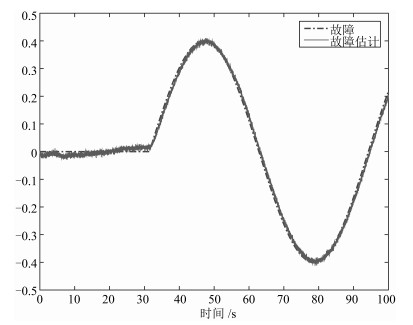 图 2 实际故障在设计频域范围内时的故障估计结果Fig. 2 Fault estimation results when the fault is actually in the designed frequency range
为了探讨所设计的有限频域故障估计器在故障频率超过设计频率$\varpi$时的性能, 在仿真中进一步考虑如下形式的故障
$ {\pmb f}(t) = \begin{cases} 0, & t <31 \mathit{\boldsymbol{s}} \\ -0.2\sin(t-31), & t\geq 31 \mathit{\boldsymbol{s}} \end{cases} $
此时的故障估计结果如图 3所示.可以看出, 在实际的故障频率太大的情况下, 故障估计器的估计准确性有所下降.这是由于故障的实际频率超出了设计范围, 导致根据有限频域范围设计的故障估计器无法达到既定的鲁棒性指标($\gamma_f=$ $0.2$).
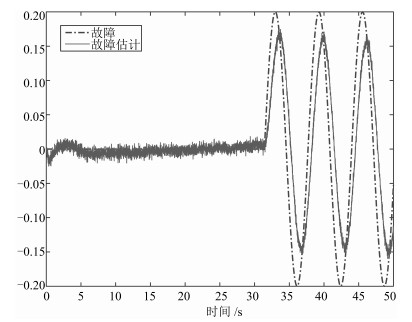 图 3 实际故障频率超出设计频域范围时的故障估计结果Fig. 3 Fault estimation results when the fault is not actually in the designed frequency range
4. 结论
本文针对具有执行器故障和未知扰动的连续线性广义系统, 提出了一种新的故障估计器设计方法.在故障属于低频范围的条件下, 利用广义KYP引理和有界实引理分析了误差系统稳定且满足给定故障估计性能指标的条件, 并且将故障估计器设计问题转化为线性矩阵不等式形式.最后通过一个受故障影响的电路系统的仿真算例说明了本文所提出方法的有效性.由文中的推导可知, 基于广义KYP引理所得到的有限频域故障估计器设计条件实际上是存在设计变量耦合的非线性矩阵不等式, 本文是通过对设计变量施加限制得到了线性矩阵不等式形式的设计条件, 因而所提出的设计方法仍然存在一定的保守性.如何进一步放宽对于设计变量的限制, 得到更为松弛的设计条件, 是有待继续研究的方向之一.
-
图 2 实际故障在设计频域范围内时的故障估计结果
Fig. 2 Fault estimation results when the fault is actually in the designed frequency range
图 3 实际故障频率超出设计频域范围时的故障估计结果
Fig. 3 Fault estimation results when the fault is not actually in the designed frequency range
表 1 不同频率范围的$\Omega$和$\Xi$
Table 1 $\Omega$ and $\Xi$ corresponding to different frequency ranges
低频范围 中频范围 高频范围 $\Omega$ $\vert \omega \vert \leq \varpi _l$ $\varpi_1\leq \omega \leq \varpi_2 $ $\vert \omega \vert \geq \varpi _h$ $\Xi$ $\left[ \begin{matrix} -\mathcal{Q} & \mathcal{P} \\ \mathcal{P} & \varpi^2_l \mathcal{Q} \end{matrix} \right] $ $\left[ \begin{matrix} -\mathcal{Q} & \mathcal{P}+j\varpi _c \mathcal{Q} \\ \mathcal{P} -j\varpi _c \mathcal{Q} & -\varpi_1\varpi_2 \mathcal{Q} \end{matrix} \right] $ $\left[ \begin{matrix} \mathcal{Q} & \mathcal{P} \\ \mathcal{P} & -\varpi^2_h \mathcal{Q} \end{matrix} \right] $  下载: 导出CSV
-
[1] Wang H, Daley S. Actuator fault diagnosis:an adaptive observer-based technique. IEEE Transactions on Automatic Control, 1996, 41(7):1073-1078 doi: 10.1109/9.508919 [2] Zhang K, Jiang B, Cocquempot V. Adaptive observer-based fast fault estimation. International Journal of Control, Automation, and Systems, 2008, 6(3):320-326 https://www.wenkuxiazai.com/doc/5c6426c6d5bbfd0a795673ad.html [3] Alwi H, Edwards C, Tan C P. Sliding mode estimation schemes for incipient sensor faults. Automatica, 2009, 45(7):1679-1685 doi: 10.1016/j.automatica.2009.02.031 [4] 张柯, 姜斌.基于故障诊断观测器的输出反馈容错控制设计.自动化学报, 2010, 36(2):274-281 http://www.aas.net.cn/CN/abstract/abstract18077.shtmlZhang Ke, Jiang Bin. Fault diagnosis observer-based output feedback fault tolerant control design. Acta Automatica Sinica, 2010, 36(2):274-281 http://www.aas.net.cn/CN/abstract/abstract18077.shtml [5] Gao Z W, Ding S X. Actuator fault robust estimation and fault-tolerant control for a class of nonlinear descriptor systems. Automatica, 2007, 43(5):912-920 doi: 10.1016/j.automatica.2006.11.018 [6] 陈莉, 钟麦英.不确定奇异时滞系统的鲁棒H∞故障诊断滤波器设计.自动化学报, 2008, 34(8):943-949 http://www.aas.net.cn/CN/abstract/abstract13517.shtmlChen Li, Zhong Mai-Ying. Designing robust H∞ fault detection filter for singular time-delay systems with uncertainty. Acta Automatica Sinica, 2008, 34(8):943-949 http://www.aas.net.cn/CN/abstract/abstract13517.shtml [7] Hamdi H, Rodrigues M, Mechmeche C, Theilliol D, Braiek N B. Fault detection and isolation in linear parameter-varying descriptor systems via proportional integral observer. International Journal of Adaptive Control and Signal Processing, 2012, 26(3):224-240 doi: 10.1002/acs.v26.3 [8] Wang Z H, Shen Y, Zhang X L. Actuator fault estimation for a class of nonlinear descriptor systems. International Journal of Systems Science, 2014, 45(3):487-496 doi: 10.1080/00207721.2012.724100 [9] Yao L N, Cocquempot V, Wang H. Fault diagnosis and fault tolerant control scheme for a class of non-linear singular systems. IET Control Theory & Applications, 2015, 9(6):843-851 http://ieeexplore.ieee.org/xpl/abstractAuthors.jsp?reload=true&arnumber=7089377 [10] Wang J L, Yang G H, Liu J. An LMI approach to H--index and mixed H-/H∞ fault detection observer design. Automatica, 2007, 43(9):1656-1665 doi: 10.1016/j.automatica.2007.02.019 [11] Yang H J, Xia Y Q, Zhang J H. Generalised finite-frequency KYP lemma in delta domain and applications to fault detection. International Journal of Control, 2011, 84(3):511-525 doi: 10.1080/00207179.2011.561501 [12] Chen J L, Cao Y Y. A stable fault detection observer design in finite frequency domain. International Journal of Control, 2013, 86(2):290-298 doi: 10.1080/00207179.2012.723829 [13] Chen J, Cao Y Y, Zhang W D. A fault detection observer design for LPV systems in finite frequency domain. International Journal of Control, 2015, 88(3):571-584 doi: 10.1080/00207179.2014.966326 [14] 李贤伟, 高会军.有限频域分析与设计的广义KYP引理方法综述.自动化学报, 2016, 42(11):1605-1619 http://www.aas.net.cn/CN/abstract/abstract18950.shtmlLi Xian-Wei, Gao Hui-Jun. An overview of generalized KYP lemma based methods for finite frequency analysis and design. Acta Automatica Sinica, 2016, 42(11):1605-1619 http://www.aas.net.cn/CN/abstract/abstract18950.shtml [15] Li X J, Yang G H. Fault detection in finite frequency domain for Takagi-Sugeno fuzzy systems with sensor faults. IEEE Transactions on Cybernetics, 2014, 44(8):1446-1458 http://ieeexplore.ieee.org/document/6650097/ [16] Long Y, Yang G H. Fault detection and isolation for networked control systems with finite frequency specifications. International Journal of Robust and Nonlinear Control, 2014, 24(3):495-514 doi: 10.1002/rnc.v24.3 [17] Ding D W, Wang H, Li X L. H--/H∞ fault detection observer design for two-dimensional Roesser systems. Systems and Control Letters, 2015, 82:115-120 doi: 10.1016/j.sysconle.2015.04.005 [18] 董全超, 钟麦英.线性时滞系统主动容错H∞控制.系统工程与电子技术, 2009, 31(11):2693-2697 http://subject.wanfangdata.com.cn/xstjbg/2010/rgzn4.htmlDong Quan-Chao, Zhong Mai-Ying. Active fault tolerant H∞ control for linear time-delay systems. Systems Engineering and Electronics, 2009, 31(11):2693-2697 http://subject.wanfangdata.com.cn/xstjbg/2010/rgzn4.html [19] Dong Q C, Zhong M Y, Ding S X. Active fault tolerant control for a class of linear time-delay systems in finite frequency domain. International Journal of Systems Science, 2012, 43(3):543-551 doi: 10.1080/00207721.2010.517862 [20] Gu Y, Ming H F, Dan Y. Fault reconstruction for linear descriptor systems using PD observer in finite frequency domain. In:Proceedings of the 24th Chinese Control and Decision Conference. Taiyuan, China:IEEE, 2012. 2281-2286 [21] Wang Z H, Rodrigues M, Theilliol D, Shen Y. Sensor fault estimation filter design for discrete-time linear time-varying systems. Acta Automatica Sinica, 2014, 40(10):2364-2369 doi: 10.1016/S1874-1029(14)60365-7 [22] Iwasaki T, Hara S. Generalized KYP lemma:unified frequency domain inequalities with design applications. IEEE Transactions on Automatic Control, 2005, 50(1):41-59 doi: 10.1109/TAC.2004.840475 [23] Wang H, Yang G H. A finite frequency domain approach to fault detection observer design for linear continuous-time systems. Asian Journal of Control, 2008, 10(5):559-568 doi: 10.1002/asjc.v10:5 [24] Gahinet P, Apkarian P. A linear matrix inequality approach to H∞ control. International Journal of Robust and Nonlinear Control, 1994, 4(4):421-448 doi: 10.1002/(ISSN)1099-1239 [25] Boyd S, Ghaoui L E, Feron E, Balakrishnan V. Linear matrix inequalities in system and control theory. Studies in Applied Mathematics. Philadelphia, PA, USA:Society for Industrial and Applied Mathematics, 1994. 7-29 期刊类型引用(4)
1. 吴小雪,丁大伟,任莹莹,刘贺平. 二维FM系统的同时故障检测与控制. 自动化学报. 2021(01): 224-234 .  本站查看
本站查看2. 王君,张晓燕,李炜. 基于事件触发机制的NNCS混合非脆弱容错控制. 信息与控制. 2019(03): 329-338 . 百度学术3. 刘蕾,路少颖,韩存武,孙德辉. 不确定时滞奇异摄动系统的最优故障估计. 北方工业大学学报. 2019(05): 69-76 . 百度学术4. 梁天添,王茂. 线性时变时滞连续-离散描述系统鲁棒故障诊断滤波器设计. 中国惯性技术学报. 2018(06): 841-848 . 百度学术其他类型引用(8)
-

 下载:
下载:

计量
- 文章访问数: 2148
- HTML全文浏览量: 244
- PDF下载量: 566
- 被引次数: 12
