

Traffic Congestion Status Identification Method for Road Network with Multi-source Uncertain Information
-
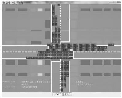
摘要: 拥堵状态辨识是道路运行状态评估的重要内容,是交通系统流量调控和管理的重要参考指标.在智能交通系统(Intelligent transport system,ITS)普及化程度越来越高的后交通时代,如何实现海量数据下对多源不确定交通拥堵状态的辨识是非常重要的内容.首先,基于多元集对分析建立一种新的路网交通拥堵状态刻画模型;然后,通过改进证据理论中Dempster组合规则实现交通信息融合,并推导出当前交通拥堵状态的准确表达值;最后,在数值模拟的基础上,使用重庆市南岸区的交通检测数据进行仿真分析,结果表明本方法能准确直观地反映出实时交通拥堵状态,具有潜在的实际应用价值.Abstract: Congestion identification is an important content of traffic condition assessment, and has significant meaning to the traffic regulation and management of transportation systems. With intelligent transport system (ITS) becoming increasingly popular, how to achieve congestion identification for uncertain multi-source information is a very important content under massive data. First, a new road network traffic congestion state characterization model is built based on multivariate set pair analysis method. Then, traffic information fusion is achieved by improving the Dempster combination rule of evidence method, and the accurate expression values of current traffic congestion are derived. Finally, the real time traffic monitoring data in Chongqing is used to verify the presented method. The results illustrate the presented method is effective, and that it is not only of theoretical significance but also of potential application value.
-
1. Introduction
For permanent magnet synchronous motor (PMSM) drive system, the measurement of instantaneous stator currents is required for successful operation of the feedback control. Generally two phase current sensors are installed in three phase voltage source inverters (VSI). Nevertheless, sudden severe failure of phase current sensors would result in over-current malfunction of the drive system. And if there is no protection scheme in the gate-drive circuit, the failure would lead to irrecoverable fault of power semiconductors in VSI, which would cause degradation of motor drive performance. Additionally, some minor failures (such as gain drift and nonzero offset) of phase current sensors would lead to torque pulsation synchronizing with the inverter output frequency [1]. The larger offset and scaling error of phase current sensors would bring about the worse performance of torque regulation. Moreover, if the offset and gain drift are above certain level, it would cause over-current trip under high speed and heavy load conditions [2]. So it is necessary to consider fault tolerant operation of phase current sensor failure.
The current sensorless technology, regarded as fault tolerant one, has been developed in the past few decades. Its core lies in that the physical fault current sensor is replaced with virtual sensor (or current estimator). This technology has several advantages such as high reliability and low cost as well as space and weight savings owing to omitting physical current sensor. Moreover, it allows the drive system to work in hostile environment.
As far as the current sensorless technique is concerned, three estimation solutions have been reported in the literature. The first one is a DC-link current-based approach which restructures phase currents with the information of the DC-link current and switching states in VSI [3]. Although it is a mainstream method, its unavoidable drawbacks are exposed: the duration of an active switching state may be so short that the DC-link current cannot be measured on one hand, on the other hand, there are immeasurable regions in the output voltage hexagon where the DC-link current sampling and reconstruction are limited or impossible to do [4]. In addition, the DC-link sensed current remains sensitive to the narrow pulse and further deteriorates if the cable capacitance causes spurious oscillations in the DC-link waveform. In order to provide high-accuracy phase current reconstruction over a wide range of operating conditions with a low current waveform, over the past years, many kinds of methods of improved PWM modulation strategy have been proposed for the single DC-link current sensor technique [5]$-$[14]. Although many improved methods show reasonable phase current reconstruction performance, these methods suffer from complicated algorithms [15]. The second one is an analytical model-based approach. In [16], on the basis of the voltage and flux equations of induction motor (IM) drive, the phase current is estimated by using the synchronous reference frame variables under single phase current sensor condition. In [17], by the discrete voltage equations of PMSM drive, the phase currents are estimated. Although it is easier to implement than the first one, the method is not robust against the variation of system parameters. The third one is an adaptive observer-based approach. In [18], the phase current is reconfigured for IM drive using single phase current sensor, while in [19], the phase currents are reconfigured for PMSM drive without any phase current sensors. Compared with the first two solutions, the third solution has stronger robustness against the variation of system parameters [20], [21]. For PMSM drive system when only one phase current sensor is available, the remaining two phase currents estimation based on an adaptive observer must be studied, which is required to perform current feedback control. However, there is no literature on such strategy.
For PMSM drive system, model predictive torque control (MPTC) is an emerging control strategy [22]$-$[29]. Its main objective is to control instantaneous torque and stator flux with high accuracy and thus MPTC plays an important role to ensure the quality of the torque and speed control. MPTC adopts the principle of model predictive control (MPC) and can provide high dynamic performance and low stator current harmonics.
For conventional proportional-integral(PI)-based MPTC PMSM drive system, its speed regulator employs the algorithm of PI. In general, PI may perform well under certain operating condition, but it does not work properly and thus degrades dynamic performance under other operating conditions such as variation of system parameters and external disturbances. To improve the robustness of the speed regulator, some techniques have been proposed in recent years [30]$-$[34]. Except these techniques, a global fast terminal sliding mode (GFTSM) control is an effective and practical one [35], [36], which is based on sliding mode theory and employs the fast terminal sliding mode in both the reaching stage and sliding stage. By adding the nonlinear function to the sliding mode surface, the GFTSM controller can enable drive system not only to be superiorly robust against system uncertainties and external disturbances but also to have quick response as well as high control precision. Even so, studies on GFTSM speed regulator are very few. In this paper, we propose replacement of PI with GFTSM for MPTC PMSM drive system.
In this paper, by referring to the adaptive approach and integrating the GFTSM method, a new GFTSM-based MPTC strategy with the adaptive observer is put forward for the PMSM drive system with single phase current sensor. The proposed adaptive observer presents a satisfactory tracking performance of the remaining two phase currents in the presence of stator resistance change caused by the temperature variation. And the designed GFTSM controller enhances the speed regulator's robustness against parameter uncertainty and external disturbance. On the basis of the above foundation, the synthesized MPTC PMSM drive control system achieves a high performance.
This paper is organized as follows: Dynamic model of PMSM drive is presented in Section 2. Section 3 gives the adaptive observer and GFTSM speed regulator design as well as MPTC design. Experimental results and analysis are presented in Section 4. Section 5 contains the conclusions.
Notation 1: The following nomenclature is used throughout this paper:
$ \begin{align*} \begin{array}{lll} R_{\rm s}:& &\mbox {Nominal phase resistance} \ \\ \psi_{\rm m}:&&\mbox{The permanent magnet flux} \ \\ \psi_{\rm s}:&&\mbox{Stator flux linkage}\\ p:&&\mbox{Number of pole pairs}\\ V_{\rm dc}:&&\mbox{DC bus voltage}\\ \omega_{\rm r}:&&\mbox{Rotor actual mechanical speed}\\ T_{\rm l}:&&\mbox{Load torque}\\ T_{\rm e}:&&\mbox{Electromagnetic torque}\\ J:&&\mbox{Moment of inertia}\\ B_{\rm m}:&&\mbox{Viscous friction coefficient}\\ T_{\rm f}:&&\mbox{Coulomb friction torque}\\ \theta:&&\mbox{Rotor electrical angular position}\\ i:&&\mbox{Stator current}\\ u:&&\mbox{Stator voltage}\\ L:&&\mbox{Stator inductance}.\\ \end{array} \end{align*} $
Notation 2: The following symbol is used throughout this paper. $\bullet_{\rm d}$, $\bullet_{\rm q}$, $\bullet_{\alpha}$ and $\bullet_{\beta}$ are used to denote the $d$-axis, $q$-axis, $\alpha$-axis, and $\beta$-axis component of $\bullet$, respectively; $\bullet^{\ast}$ is used to denote the reference values of $\bullet$; $\hat{\bullet}$ is used to denote the estimate of $\bullet$; $\tilde{\bullet}$ is used to denote the parameter estimation error of $\bullet$; $\bullet^{k}$ and $\bullet^{k+1}$ are used to denote the instantaneous value at $k$th and ($k+1$)th of $\bullet$, respectively.
2. Dynamic Models of Three-phase PMSM Drive
As for three-phase PMSM drive, the models in rotor synchronous reference frame ($dq$-frame) and two-phase stationary reference frame ($\alpha\beta$-frame) are expressed as follows, respectively:
$ \begin{align} \label{eq:1} % eq:(1) \begin{cases} \dfrac{{d}i_{\rm d}}{{d}t}&=\dfrac{1}{L_{\rm d}} \left(u_{\rm d}-R_{\rm s}i_{\rm d}+p\omega_{\rm r}L_{\rm q}i_{\rm q}\right) \\[3mm] \dfrac{{d}i_{\rm q}}{{d}t}&=\dfrac{1}{L_{\rm q}}\left(u_{\rm q}-R_{\rm s}i_{\rm q}+p\omega_{\rm r} (L_{\rm d}i_{\rm d}+\psi_{\rm m})\right) \end{cases}\end{align} $
(1) $\begin{align} \begin{cases} \dfrac{{d}i_{\alpha}}{{d}t}&=\dfrac{1}{L_{\alpha}} \left(u_{\alpha}-R_{\rm s}i_{\alpha}+p\omega_{\rm r}\psi_{\rm m} \sin\theta\right) \\[3mm] \dfrac{{d}i_{\beta}}{{d}t}&=\dfrac{1}{L_{\beta}} \left(u_{\beta}-R_{\rm s}i_{\beta}-p\omega_{\rm r}\psi_{\rm m}\cos\theta\right) \end{cases} \end{align} $
(2) and the mechanical equation is expressed as
$ \begin{align} \dfrac{{d}\omega_{\rm r}}{{d}t}=\dfrac{1}{J}(T_{\rm e}-T_{\rm l}-B_{\rm m}\omega_{\rm r}-T_{\rm f}) \end{align} $
(3) where the electromagnetic torque $T_{\rm e}$ is expressed as
$\begin{align} T_{\rm e}=\frac{3{ p}}{2} \left[\psi_{\rm m}i_{\rm q}+(L_{\rm d}-L_{\rm q})i_{\rm d}i_{\rm q}\right]. \end{align} $
(4) 3. Design of GFTSM-based MPTC PMSM Drive System With Adaptive Observer
The objective of GFTSM-based MPTC using adaptive observer is that the PMSM drive system can work reliably and its speed and torque can be controlled not only to have satisfactory performance but also to be strongly robust against parameters variation and external disturbance. The schematic of the proposed control system is shown in Fig. 1. Our design task concentrates on adaptive observer, GFTSM speed regulator and MPTC as follows.
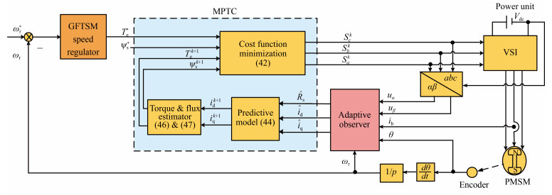 图 1 Block diagram of GFTSM-based MPTC PMSM drive system with adaptive observer.Fig. 1 Block diagram of GFTSM-based MPTC PMSM drive system with adaptive observer.
3.1 Adaptive Observer Design
The proposed adaptive observer is to estimate the remaining two phase currents and stator resistance when single phase current sensor is available. In the design process, assume the following conditions.
1) Only phase-$b$ current can be measured and the remaining two phase current sensors are not available.
2) Due to heating during operating of the motor, the stator resistance $R_{\rm s}$ is considered as a time-varying parameter.
3) There is no saturation in the magnetic circuit.
For surface-mounted PMSM drive, $L_{\rm d}=L_{\rm q}=L_{\alpha}= L_{\beta}$ $=$ $L$. The $\alpha$-axis in $\alpha\beta$-frame is oriented along phase-$a$ axis in three-phase stationary reference frame ($abc$-frame). The $abc$-axis stator currents in $abc$-frame can be obtained from the $\alpha\beta$-axis ones in $\alpha\beta$-frame by the following transformation matrix:
$ \left[ \begin{matrix} {{i}_{\rm{a}}} \\ {{i}_{\rm{b}}} \\ {{i}_{\rm{c}}} \\ \end{matrix} \right]=\left[ \begin{matrix} 1 & 0 \\ -\frac{1}{2} & \frac{\sqrt{3}}{2} \\ -\frac{1}{2} & -\frac{\sqrt{3}}{2} \\ \end{matrix} \right]\left[ \begin{matrix} {{i}_{\alpha }} \\ {{i}_{\beta }} \\ \end{matrix} \right] $
(5) where $i_{\rm a}$, $i_{\rm b}$, and $i_{\rm c}$ are $abc$-axis stator currents in $abc$-frame. From (5), the following equation can be given,
$ \begin{align} % eq:(6) i_{\rm b}=-\frac{1}{2} i_\alpha+\frac{\sqrt{3}}{2}i_\beta. \end{align} $
(6) Taking (2) into account, the time derivative of (6) is deduced as follows:
$ \begin{align} % eq:(7) \frac{{d}i_{\rm b}}{{d}t}& =\dfrac{\sqrt{3}}{2L}\left[u_\beta-R_{\rm s}\left(\frac{1}{ \sqrt{3}}i_\alpha+\frac{2}{ \sqrt{3}}i_{\rm b}\right)-p\omega_{\rm r}\psi_m\cos\theta\right]\notag\\ & \quad -\frac{1}{2L} (u_{\alpha}-R_{\rm s}i_{\alpha}+p\omega_{\rm r}\psi_{\rm m}\sin\theta)\notag\\ &=\frac{\sqrt{3}u_\beta-u_{\alpha}-2R_{\rm s}i_{\rm b}-p\omega_{\rm r}\psi_{\rm m}(\sqrt{3}\cos\theta+\sin\theta)} {2L}. \end{align} $
(7) The following adaptive observer is proposed in order to estimate phase-$b$ current,
$ \begin{align} % eq:(8) \frac{{d}\hat{i}_{\rm b}}{{d}t}& =\frac{\sqrt{3}}{ 2L}\left[u_\beta-\hat{R}_{\rm s}\left(\frac{1}{ \sqrt{3}}\hat{i}_\alpha+\frac{2}{ \sqrt{3}}i_{\rm b}\right)-p\omega_{\rm r}\psi_m\cos\theta\right]\notag\\ & \quad -\frac{1}{ 2L}\left(u_{\alpha}-\hat{R}_{\rm s}\hat{i}_{\alpha}+p\omega_{\rm r}\psi_{\rm m}\sin\theta\right)-k_1f(\tilde{i}_{\rm b})-k_2\tilde{i}_{\rm b}\notag\\ & =\frac{1}{2L}\left[\sqrt{3}u_\beta-u_{\alpha}-2\hat{R}_{\rm s}i_{\rm b}-p\omega_{\rm r}\psi_{\rm m}(\sqrt{3}\cos\theta + \sin\theta)\right]\notag\\ &\quad-k_1f(\tilde{i}_{\rm b})-k_2\tilde{i}_{\rm b} \end{align} $
(8) where $k_1f(\tilde{i}_{\rm b})$ and $k_2\tilde{i}_{\rm b}$ are correctors, and $k_1$ and $k_2$ are the positive observer gains, and $f(\cdot)$ denotes the nonlinear function of phase-$b$ current estimation error $\tilde{i}_{\rm b}$, which is defined as
$ \begin{align} % eq:(9) \tilde{i}_{\rm b}=\hat{i}_{\rm b}-i_{\rm b}. \end{align} $
(9) Define the following stator resistance estimation error,
$ \begin{align} % eq:(10) \tilde{R}_{\rm s}=\hat{R}_{\rm s}-R_{\rm s}. \end{align} $
(10) By subtracting (8) from (7), the dynamics equation of the phase-$b$ current estimation error is given as follows:
$ \begin{align} % eq:(11) \frac{{d}\tilde{i}_{\rm b}}{{d}t}=-\frac{1}{ L}\tilde{R}_{\rm s}i_{\rm b}-k_1f(\tilde{i}_{\rm b})-k_2\tilde{i}_{\rm b}. \end{align} $
(11) In order to determine the adaptive law of the stator resistance and the observer gains, construct the candidate Lyapunov function as
$ \begin{align} % eq:(12) V_1=\frac{1}{ 2}\left(\tilde{i}_{\rm b}^2+{1\over r}\tilde{R}_{\rm s}^2\right) \end{align} $
(12) where $r$ is constant positive scalar.
The time derivative of (12) is obtained as follows:
$ \begin{align} % eq:(13) \frac{{d}{V_1}}{{d}t}=-k_2\tilde{i}_{\rm b}^2-k_1f(\tilde{i}_{\rm b})\tilde{i}_{\rm b}+\tilde{R}_{\rm s}\left(\frac{1}{ r}\frac{{d}\tilde{R}_{\rm s}}{{d}t}-\frac{1}{ L}i_{\rm b}\tilde{i}_{\rm b}\right). \end{align} $
(13) If we define following equality,
$ \begin{align} % eq:(14) \frac{1}{r}\frac{{d}\tilde{R}_{\rm s}}{{d}t}-\frac{1}{ L}i_{\rm b}\tilde{i}_{\rm b}=0. \end{align} $
(14) Equation (13) can be rewritten as below:
$ \begin{align} % eq:(15) \frac{{d}{V_1}}{{d}t}=-k_2\tilde{i}_{\rm b}^2-k_1f(\tilde{i}_{\rm b})\tilde{i}_{\rm b}. \end{align} $
(15) To render $\dot V_{1}$ negative, we assume
$ \begin{align} % eq:(16) f(\tilde{i}_{\rm b})={\rm sign}(\tilde{i}_{\rm b}). \end{align} $
(16) As a result, the following inequality is satisfied
$ \frac{{d}{V_1}}{{d}t}<0. $
By Lyapunov stability theorem, dynamic system (11) is stable, which means that both $\tilde{i}_{\rm b}$ and $\tilde{R}_{\rm s}$ can converge to zero. Since the variation of the stator resistance in the observer time scale is negligible, i.e.,
$ \frac{{d}R_{\rm s}}{{d}t}\approx 0 $
then the following formula holds
$ \begin{align} % eq:(17) \frac{{d}\tilde{R}_{\rm s}}{{d}t}=\frac{{d}\hat{R}_{\rm s}}{{d}t}-\frac{{d}R_{\rm s}}{{d}t}\approx\frac{{d}\hat{R}_{\rm s}}{{d}t}. \end{align} $
(17) Therefore, from (14), the adaptive mechanism of the stator resistance is derived as follows:
$ \begin{align} % eq:(18) \hat{R}_{\rm s}={r\over L}\int(i_{\rm b}\tilde{i}_{\rm b}){ d}t. \end{align} $
(18) With the adaptive mechanism in (18), the estimation value of the stator resistance can converge to its real value.
In order to improve the estimation accuracy of the stator resistance and to ensure a null steady error, on the basis of PI strategy, (18) is modified as below:
$ \begin{align} % eq:(19) \hat{R}_{\rm s}=\frac{r}{ L}\left\{{K_{P(R_{\rm s})}[i_{\rm b}(\hat{i}_{\rm b}-i_{\rm b})]+K_{I(R_{\rm s})}\int[i_{\rm b}(\hat{i}_{\rm b}-i_{\rm b})]{d}t}\right\} \end{align} $
(19) where $K_{P(R_{\rm s})}$ and $K_{I(R_{\rm s})}$ are proportional and integral scalars, respectively.
By replacing $R_{\rm s}$ in (2) with $\hat{R}_{\rm s}$ in (19), the $\alpha\beta$-axis currents observers can be constructed as follows:
$ \begin{align} % eq:(20) \begin{cases} \dfrac{{d}\hat{i}_{\alpha}}{{d}t}=\dfrac{1}{ L} \left(u_{\alpha}-\hat{R}_{\rm s}\hat{i}_{\alpha}+p\omega_{\rm r} \psi_{\rm m}\sin\theta\right) \\[3mm] \dfrac{{d}\hat{i}_{\beta}}{{d}t} =\dfrac{1}{ L}\left(u_{\beta}-\hat{R}_{\rm s}\hat{i}_{\beta} -p\omega_{\rm r}\psi_{\rm m}\cos\theta\right). \end{cases} \end{align} $
(20) By combining (8), (19) and (20), the block diagram of the designed adaptive observer is established as shown in Fig. 2, which treats the stator voltages, rotor electrical position and speed as the inputs, the $dq$-axis currents and stator resistance as outputs when only phase-$b$ current is measured.
 图 2 Block diagram of the proposed adaptive observer.Fig. 2 Block diagram of the proposed adaptive observer.
Remark 1: From Fig. 2, it can be seen that estimating the phase-$b$ current is a key step and primary premise in construction of the adaptive observer. The error between the phase-$b$ measured current and its estimated value must be guaranteed to converge towards zero.
Remark 2: From (8) and (19), it can be seen that although the coupling relationship between $\hat{i}_{\rm b}$ and $\hat{R}_{\rm s}$ exists, we do not need to decouple them in the design process. In fact, the phase-$b$ current estimation (8) and the stator resistance adaptive law (19) are implemented and solved all together.
Remark 3: The convergence rate of the observer is dependent on the observer gains $k_1$ and $k_2$, which should be chosen to be large enough such that the observer responds as soon as possible.
Remark 4: The estimated $dq$-axis currents in Fig. 2 will be applied to MPTC as shown in Fig. 1.
Remark 5: From (5), the estimation of phase-$a$ current in $abc$-frame is equal to that of $\alpha$-axis current in $\alpha\beta$-frame as follows:
$ \begin{align} % eq:(21) \hat{i}_{\rm a}=\hat{i}_{\alpha}. \end{align} $
(21) Accordingly, the estimation of phase-$c$ current in $abc$-frame can be obtained as follows:
$ \hat{i}_{\rm c}=-(i_{\rm b}+\hat{i}_{\alpha}). $
Remark 6: The proposed adaptive observer is robust against only the stator resistance change. If other parameter uncertainties (such as stator inductance change and permanent magnet flux change, etc.) and unmodeled dynamics are required to be considered, then adaptive robust method with extended state observer can be borrowed from [20] and [33], which is our next research topic.
3.2 GFTSM Speed Regulator Design
3.2.1 GFTSM Design
Define the speed error as
$ e=\omega_{\rm r}^{\ast}-\omega_{\rm r}. $
Let
$ \begin{align} % eq:(22) x_1=e, ~~x_2=\dot{x}_{1}, ~~ u=\dot{T}_{\rm e}. \end{align} $
(22) Assume that $\omega_{\rm r}^{\ast}$ (or $\dot{\omega}_{\rm r}^{\ast}$), $T_{\rm l}$, $T_{\rm f}$ are constants and $\omega_{\rm r}$ has continuous second-order derivative. Then, the state equation of (3) can be expressed as following:
$ \begin{align} % eq:(23) \begin{cases} \dot{x}_{1}=x_2\\[1mm] \dot{x}_{2}=-\dfrac{B_{\rm m}}{ J}x_2-\dfrac{1}{ J}u \end{cases} \end{align} $
(23) where $u$ can be regarded as the control input.
Our target is to enable the drive system to be strongly robust and to have very fast response. For this reason, based on sliding mode theory, GFTSM speed regulator is employed. Fast terminal sliding mode surface is designed as following:
$ \begin{align} % eq:(24) s=\dot{x}_{1}+\alpha x_{1}+\beta x_{1}^\frac{q}{p} \end{align} $
(24) where $\alpha$, $\beta>0$; $q$, $p$ $(q<p)$ are positive odd integers.
Taking the first-order derivative of (24) yields
$ \begin{align} % eq:(25) \dot{s}=\left(\alpha-\frac{B_{\rm m}}{ J}\right)x_2-{\frac{1}{ J}}u+\beta\frac{{d}}{{d}t}\left(x_{1}^\frac{q}{p}\right). \end{align} $
(25) To make the system (23) reach the sliding mode surface in finite time, the fast terminal attractor is adopted as follows:
$ \begin{align} % eq:(26) \dot{s}=-\varphi s-\gamma s^\frac{v}{m} \end{align} $
(26) where $\varphi>0$, $\gamma>0$, $m>0$, $v>0$; $m$ and $v$ are odd integers.
Let (25) be equal to (26) and thus the following sliding mode control law can be obtained
$ \begin{align} % eq:(27) u=J\left(\left(\alpha-\frac{B_{\rm m}}{ J}\right)x_2+\beta\frac{{d}}{{d}t}\left(x_{1}^\frac{q}{p}\right)+\varphi s+\gamma s^\frac{v}{m}\right). \end{align} $
(27) By combining (23), (24) and (27), the block diagram of the designed GFTSM speed regulator is shown as in Fig. 3.
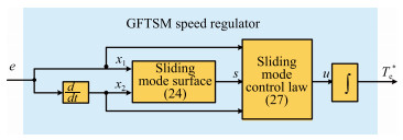 图 3 Block diagram of the designed GFTSM speed regulator.Fig. 3 Block diagram of the designed GFTSM speed regulator.
By solving differential equation (26), the time from any state $s(0)\neq 0$ to the sliding mode surface $s(t_f)$ can be derived as follows:
$ \begin{align} % eq:(28) t_f=\frac{m}{ \varphi(m-v)}\ln\frac{\varphi\left(s(0)\right)^\frac{m-v}{m}+\gamma}{ \gamma}. \end{align} $
(28) Remark 7: From (27), it can be seen that the sliding mode control law does not include switching item and thus weakens system chatter.
Remark 8: Under control law (27), one can easily see that if it converges to zero according to the terminal attractor (26), $x_1$ will accordingly converge to zero in terms of the following fast terminal attractor
$ \begin{align} % eq:(29) \dot{x}_{1}=-\alpha x_{1}-\beta x_{1}^\frac{q}{p}. \end{align} $
(29) It can be observed from (26) and (29) that the fast terminal attractors are adopted both in the reaching phase and in sliding phase. Consequently, the designed regulator (27) is a global terminal sliding mode one which guarantees the finite time control performance.
Remark 9: According to (28), $t_f$ can be set arbitrarily by adjusting parameters $m$, $v$, $\varphi$, $\gamma$.
Remark 10: The designed GFTSM speed regulator (27) is not only stable but also robust, which will be analyzed as below.
3.2.2 Stability Analysis
Construct Lyapunov function as
$ \begin{align} % eq:(30) V_2=\frac{1}{2}s^{2}. \end{align} $
(30) Differentiating (30) yields
$ \dot{V}_2=s\dot{s}=-\varphi s^2-\gamma s^\frac{m+v}{m} $
since $(m+v)$ is an even number, therefore $\dot{V}=s\dot{s}<0$. According to Lyapunov stability theory, the system (23) is stable and its movement can tend to sliding mode surface and finally reach the sliding mode.
3.2.3 Robustness Analysis
Considering parameter uncertainties and external disturbances, the system (23) is rewritten as following:
$\begin{align} % eq:(31) \begin{cases} \dot{x}_{1}=x_2\\[1mm] \dot{x}_{2}=-\dfrac{B_{\rm m}}{ J}x_2-\dfrac{1}{ J}u+d(x_1, x_2) \end{cases} \end{align} $
(31) where $d(x_1, x_2)$ can be regarded as the total disturbance including uncertainties and external disturbances. Assume $| d(x_1, x_2)|$ $\leq$ $D$, $D$ is maximum value.
As for system (31), differentiating (24) yields
$ \begin{align} % eq:(32) \dot{s}=\left(\alpha-\frac{B_{\rm m}}{ J}\right)x_2-\frac{1}{ J}u+d(x_1, x_2)+\beta\frac{{d}}{{d}t}\left(x_{1}^\frac{q}{p}\right). \end{align} $
(32) Substituting (27) into (32) yields
$ \begin{align} % eq:(33) \dot{s}& =-\varphi s-\gamma s^\frac{v}{m}+d(x_1, x_2)\notag\\[1mm] & =-\varphi s-\left(\gamma-\frac{d(x_1, x_2)} {s^\frac{v}{m}}\right)s^\frac{v}{m}. \end{align} $
(33) Let
$ \begin{align} % eq:(34) \bar{\gamma}=\gamma-\frac{d(x_1, x_2)}{s^\frac{v}{m}} \end{align} $
(34) then (33) can be rewritten as
$ \begin{align} % eq:(35) \dot{s}=-\varphi s-\bar{\gamma} s^\frac{v}{m}. \end{align} $
(35) To make (35) be a fast terminal attractor, (34) must satisfy $\bar{\gamma}>0$. Therefore, the following inequality holds true
$ \gamma-\frac{d(x_1, x_2)}{s^\frac{v}{m}}>\gamma-\frac{| d(x_1, x_2)|}{| s^\frac{v}{m}|}>\gamma-\frac{D}{ | s^\frac{v}{m}|}>0 $
then we can deduce
$ \begin{align} % eq:(36) \gamma>\frac{D}{ | s^\frac{v}{m}|}. \end{align} $
(36) Equation (36) is equivalent to
$ \begin{align} % eq:(37) | s|>\left(\frac{D}{ \gamma }\right)^\frac{m}{v}. \end{align} $
(37) As a result, the fast terminal convergence region $\Delta$ is constrained by
$ \begin{align} % eq:(38) \Delta=\left\{x_1, x_2:| s|\leq \left(\frac{D}{ \gamma }\right)^\frac{m}{v}\right\}. \end{align} $
(38) Furthermore, we assume
$ \begin{align} % eq:(39) \gamma={D\over | s^\frac{v}{m}|}+\eta, ~~~\eta>0. \end{align} $
(39) According to (35), the time from any state $s(0)\neq 0$ to the sliding surface is deduced as follows:
$ \begin{align} % eq:(40) \bar{t}_f={m\over \varphi(m-v)}\ln{\varphi\left(s(0)\right)^\frac{m-v}{m}+\bar{\gamma}\over \bar{\gamma}}. \end{align} $
(40) Since $\bar{\gamma}>\eta$, the following inequality can be deduced
$ \ln\frac{\varphi\left(s(0)\right)^\frac{m-v}{m}+\bar{\gamma}}{ \bar{\gamma}}\leq \ln\frac{\varphi\left(s(0)\right)^\frac{m-v}{m}+\eta}{ \eta} $
and then the reaching time satisfies
$ \begin{align} % eq:(41) \bar{t}_f\leq\frac{m}{ \varphi(m-v)}\ln\frac{\varphi\left(s(0)\right)^\frac{m-v}{m}+\eta}{ \eta}. \end{align} $
(41) Through the above analysis, it can be seen that if the condition $\bar{\gamma}>0$ holds then fast terminal convergence can be guaranteed and system (31) can reach neighborhood $\Delta$ of the sliding mode surface $s(\bar{t}_f)=0$ in finite time $\bar{t}_f$.
3.3 Model Predictive Torque Control
The basic idea of MPTC is to predict the future behavior of the variables over a time frame based on the model of the system. As shown in Fig. 1, MPTC includes three parts: cost function minimization, predictive model and flux and torque estimator.
3.3.1 Cost Function Minimization
For MPTC, the cost function is chosen such that both torque and flux at the end of the cycle is as close as possible to the reference value. Generally, the minimum value of cost function is defined as
$ \begin{align} % eq:(42) &\min g =\left| T_{\rm e}^{\ast}-T_{\rm e}^{k+1}\right|+k_3\left| \left| \psi_{\rm s}^{\ast}\right|-| \psi_{\rm s}^{k+1}| \right|\notag \\ &\, {\rm s.t.}\quad u_{\rm s}^{k}\in\{V_1, V_2, \ldots, V_6\} \end{align} $
(42) where $V_1$, $V_2$, $V_3$, $V_4$, $V_5$, and $V_6$ are six nonzero voltage space vectors and can be generated by three phase VSI with respect to the different switches states. A set of voltage space vectors $u_{\rm s}^{k}$ at $k$th instant is defined as
$ \begin{align} % eq:(43) u_{\rm s}^{k}=\frac{2V_{\rm dc}\left[S_{\rm a}^{k}+e^\frac{i2\pi}{3}S_{\rm b}^{k}+(e^\frac{i2\pi}{3})^{2}S_{\rm c}^{k}\right]}{3} \end{align} $
(43) where $S_{\rm a}^{k}~(x=a, b, c)$ at $k$th instant is upper power switch state of one of three legs. $S_{\rm a}^{k}=1$ or $S_{\rm a}^{k}=0$ when upper power switch of one leg is on or off. $k_3$ is the weighting factor.
In order to compensate inherent one-step delay which exists in practical digital system, the cost function (42) is revised as below:
$ \begin{align} % eq:(44) &\min g =\left| T_{\rm e}^{\ast}-T_{\rm e}^{k+2}\right|+k_3\left| \left| \psi_{\rm s}^{\ast}\right|-| \psi_{\rm s}^{k+2}| \right|\notag \\ &\, {\rm s.t.}\quad u_{\rm s}^{k}\in\{V_1, V_2, \ldots, V_6\}. \end{align} $
(44) 3.3.2 Predictive Model for Stator Currents
According to (1), the prediction of the stator current at the next sampling instant is expressed as
$ \begin{align} % eq:(45) \begin{cases} i_{\rm d}^{k+1}=i_{\rm d}^{k}+\dfrac{1}{L}\left(u_{\rm d}^{k}-R_{\rm s}i_{\rm d}^{k}+p\omega_{\rm r}^{k}Li_{\rm q}^{k}\right)T_{\rm s}\\[3mm] i_{\rm q}^{k+1}=i_{\rm q}^{k}+\dfrac{1}{ L}\left (u_{\rm q}^{k}-R_{\rm s}i_{\rm q}^{k}-p\omega_{\rm r}^{k} (Li_{\rm d}^{k}+\psi_{\rm m})\right)T_{\rm s} \end{cases} \end{align} $
(45) where $i_{\rm d}^{k}$, $i_{\rm q}^{k}$ and $R_{\rm s}$ are replaced by the corresponding estimated values coming from the observer in Fig. 2. $T_{\rm s}$ is the sampling period.
3.3.3 Torque and Flux Estimators
In $dq$-frame, the current-based flux-linkage can be expressed as following vector:
$ \begin{align} \left[% eq:(46) \begin{array}{c} \psi_{\rm d}^{k+1} \\ \psi_{\rm q}^{k+1} \\ \end{array} \right]=\left[ \begin{array}{cc} L&0 \\ 0&L \\ \end{array} \right]\left[ \begin{array}{c} i_{\rm d}^{k+1} \\ i_{\rm q}^{k+1}\\ \end{array} \right]+\left[ \begin{array}{c} \psi_{\rm m} \\ 0 \\ \end{array} \right]. \end{align} $
(46) The magnitude of stator flux linkage $\psi_{\rm s}$ is
$ \begin{align} % eq:(47) \psi_{\rm s}^{k+1}=\sqrt{(\psi_{\rm d}^{k+1})^2+(\psi_{\rm q}^{k+1})^2}. \end{align} $
(47) Electromagnetic torque developed in $dq$-frame can be estimated as following:
$ \begin{align} % eq:(48) T_{\rm e}^{k+1}=\frac{3}{ 2}{ p}\psi_{\rm m}i_{\rm q}^{k+1}. \end{align} $
(48) Substituting (45) into (48), the torque can be calculated.
4. Simulation Result and Analysis
In order to validate the effectiveness of proposed control strategy, the designed control system as shown in Fig. 1 has been implemented in MATLAB/Simulink/Simscape platform. The parameters of PMSM drive are given in Table Ⅰ. The sampling period is 100 $\mu$s, and value $k_3$ is selected to be 200. The reference stator flux $\psi_{\rm s}^{\ast}$ is 0.175 Wb. The parameters of the adaptive observer are
$ \begin{align*} &K_{P(R_{\rm s})}=0.006, ~~~K_{I(R_{\rm s})}=8\\ &k_1=30, ~~~k_2=5000, ~~~r=1000. \end{align*} $
表 Ⅰ PARAMETERS OF PMSM DRIVETable Ⅰ PARAMETERS OF PMSM DRIVESymbol Value Symbol Value $R_{\rm s}$ $2.875\, \Omega$ $\omega_{\rm r}^{\ast}$ 1000 rpm $L_{\rm d}, L_{\rm q}$ 0.0085 H $T_{\rm n}$ 4 N$\cdot$m $\psi_{\rm m}$ 0.175 Wb $J$ $0.0008\, {\rm Kg\cdot m}^2$ $p$ 4 $B_{\rm m}$ 0.001 N$\cdot$m$\cdot$s $V_{\rm dc}$ 300 V $T_{\rm f}$ 0 The parameters of GFTSM in Fig. 3 are determined as follows:
$ \begin{align*} &\alpha=100, ~~~\beta=250, ~~~p=7, ~~~q=5\\ &\varphi=1000, ~~~\gamma=80\, 000, ~~~ m=3, ~~~v=1.\end{align*} $
4.1 The GFTSM-based MPTC PMSM Drive System Comparison Between the One With Single Phase Current Sensor and the Other With Two Phase Current Sensors
In order to verify estimation accuracy of the observer for GFTSM-based MPTC PMSM drive system with single phase current sensor, two scenarios of numerical simulation are provided and compared, which correspond to PMSM system with two phase current sensors (phase-$a$ and -$b$ sensors) and PMSM system with single phase current sensor (phase-$b$), respectively. For convenience sake, the former scenario is marked as Case 1 and the latter one as Case 2. Except the above-mentioned different number of current sensors, the two systems employ completely identical GFTSM-based MPTC strategy.
Fig. 4 shows comparison of two scenarios in terms of stator currents, stator resistance, rotor speed and torque when the reference speed $n^{\ast}$ is set to 1000 pm, the load torque is increased from 0 N$\cdot$m to 4 N$\cdot$m at 0.1 seconds and the stator resistance is changed from its nominal value 2.875 $\Omega$ to 5 $\Omega$ at 0.3 seconds.
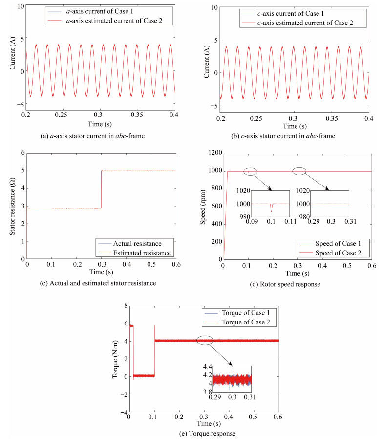 图 4 Dynamic response comparison between Case 1 and Case 2 under the variation of stator resistance.Fig. 4 Dynamic response comparison between Case 1 and Case 2 under the variation of stator resistance.
From Figs. 4(a)$-$4(c), it can be seen that, for designed adaptive observer of Case 2, its estimated $a$-axis and $c$-axis currents in $abc$-frame rapidly track corresponding ones of Case 1, and its estimated stator resistance can rapidly follow actual resistance change and converge to its actual value accurately. Figs. 4(d)$-$4(e) show that, for GFTSM-based MPTC system of Case 2, its speed and torque can be regulated in a satisfactory manner and it has almost as good performance as GFTSM-based MPTC system of Case 1.
4.2 The MPTC PMSM System Comparison Between the One Based on PI and the Other Based on GFTSM
For GFTSM-based MPTC PMSM systems, for the sake of verifying its stronger robustness, two systems are compared, which correspond to the PI-based and GFTSM-based MPTC PMSM systems, respectively. Except distinct outer-loop speed regulator (i.e., PI and GFTSM), the two systems employ completely identical MPTC and adaptive observer. In the simulation, their reference speeds $n^{\ast}$ are set to 1000 rpm, their load torques of 0 N$\cdot$m are increased to 4 N$\cdot$m at 0.1 seconds and stator resistance is at its nominal value 2.875 $\Omega$.
In the simulation, sampling values of three-phase currents are recorded over the time range from 0.1 seconds to 0.2 seconds. During this period, the fundamental frequency of three-phase currents is 66.67 Hz. Total harmonic distortion (THD) can be obtained by comparing the higher frequency components to the fundamental one.
4.2.1 The Comparison of Anti-load Variation Ability Under the Same Speed Transient Response
The parameters of PI for PI-based MPTC PMSM system are adjusted as follows:
$ K_P=0.7, ~~~K_I=0.03 $
such that PI-based MPTC system has almost the same speed transient response as GFTSM-based one.
Fig. 5 shows the dynamical responses in terms of speed, torque and stator currents. Fig. 5(a) intuitively gives the speed response comparison, which demonstrates that for GFTSM-based MPTC PMSM system, its speed can sharply adapt to the change of external load in a satisfactory manner, and its capability of accommodating the challenge of load disturbance is superior to PI-based one's. From Figs. 5(b)$-$5(d), it can be observed that for two systems with same adaptive observer, their torques, estimated $a$-axis and $c$-axis currents in $abc$-frame are almost the same.
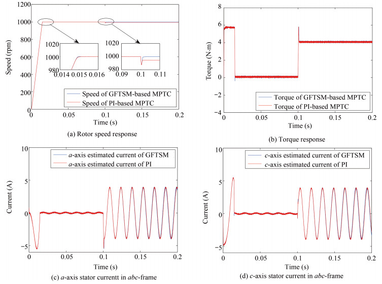 图 5 The comparison of anti-load variation ability under the same speed transient response.Fig. 5 The comparison of anti-load variation ability under the same speed transient response.
Table Ⅱ shows THD comparison of three-phase currents. From Table Ⅱ, what can be observed is that the THD of the GFTSM-based MPTC is smaller than one of the PI-based MPTC.
表 Ⅱ THD OF THREE-PHASE STATORS' CURRENT(%)Table Ⅱ THD OF THREE-PHASE STATORS' CURRENT(%)Control scheme $i_{\rm a}$ $i_{\rm b}$ $i_{\rm c}$ PI-based MPTC $2.21$ $2.32$ $2.24$ GFTSM-based MPTC $1.84$ $1.88$ $1.85$ 4.2.2 The Comparison of Dynamic Responses Under the Same Speed Anti-load Variation Ability
The parameters of PI for PI-based MPTC PMSM system are adjusted as follows:
$ K_P=3, ~~~K_I=0.1 $
such that PI-based MPTC system has almost the same anti-load variation ability as GFTSM-based one.
Figs. 6(a)$-$6(d) show the dynamical responses in terms of speed, torque and stator currents. Fig. 6(a) intuitively gives their speed response comparison, which indicates that GFTSM-based MPTC PMSM system has smaller overshoot and faster settling time than PI-based one. Meanwhile, it can be found from Fig. 6(b) that the torque response of GFTSM-based MPTC PMSM system is better than one of PI-based. From Figs. 6(c)$-$6(d), it can be observed that, their estimated $a$-axis and $c$-axis currents in $abc$-frame are almost the same.
 图 6 The comparison of dynamical response under the same speed anti-load variation ability.Fig. 6 The comparison of dynamical response under the same speed anti-load variation ability.
4.3 The MPTC PMSM System Comparison Between the One Based on SM and the Other Based on GFTSM
Here, the working condition of PMSM drive system is identical with Section 4.2.
For SM-based speed regulator, its sliding mode surface and its reaching law are selected as following:
$ s=ce+\dot{e} $
(49) $ \dot{s}=-k_4s-\varepsilon {\rm sign}(s) $
(50) 4.3.1 The Comparison of Anti-load Variation Ability Under the Same Speed Transient Response
The parameters of SM for SM-based MPTC PMSM system are adjusted as follows:
$ c=160, ~~~k_4=800, ~~~\varepsilon=3\times 10^5 $
such that SM-based MPTC system has almost the same speed transient response as GFTSM-based one.
Figs. 7(a)$-$7(d) show the dynamical responses in terms of speed, torque and stator currents. Fig. 7(a) illustrates that for GFTSM-based MPTC PMSM system, benefiting from the fast terminal sliding mode employed in both the reaching stage and the sliding stage, its recovery rate of speed response is obviously faster than SM-based one. From Figs. 7(b)$-$7(d), it can be seen that for two systems with same adaptive observer, their torques, estimated $a$-axis and $c$-axis currents in $abc$-frame are almost the same.
 图 7 The comparison of anti-load variation ability under the same speed transient response.Fig. 7 The comparison of anti-load variation ability under the same speed transient response.
Table Ⅲ shows THD comparison of three-phase currents. From Table Ⅲ, what can be observed is that the THD of the GFTSM-based MPTC is smaller than one of the SM-based MPTC.
表 Ⅲ THD OF THREE-PHASE STATORS' CURRENT(%)Table Ⅲ THD OF THREE-PHASE STATORS' CURRENT(%)Control scheme $i_{\rm a}$ $i_{\rm b}$ $i_{\rm c}$ SM-based MPTC $2.01$ $2.12$ $2.14$ GFTSM-based MPTC $1.84$ $1.88$ $1.85$ 4.3.2 The Comparison of Dynamic Response Under the Same Speed Anti-load Variation Ability
The parameters of SM for SM-based MPTC PMSM system are adjusted as follows:
$ c=140, ~~k_4=2500, ~~\varepsilon=3\times 10^7 $
such that SM-based MPTC system has almost the same anti-load variation ability as GFTSM-based one.
Figs. 8(a)$-$8(d) show the dynamical responses in terms of speed, torque and stator currents. Fig. 8(a) shows that the speed dynamic performance is better than SM-based one. And it can be found from Figs. 8(b)$-$8(d) that for SM-based MPTC PMSM system, due to a switching function sign$(\cdot)$ in (50), therefore its torque, estimated $a$-axis and $c$-axis currents have significantly heavy chatter. On the other hand, for GFTSM-based one, its sliding reaching law in (26) is a continuous and smooth function, so the system chatter can be greatly reduced.
 图 8 The comparison of dynamic response under the same anti-load variation ability.Fig. 8 The comparison of dynamic response under the same anti-load variation ability.
Summarizing above simulation experiments, we can obtain following results,
1) The proposed adaptive observer can estimate the remaining two phase currents and stator resistance rapidly and accurately.
2) Compared with PI-based and SM-based MPTC PMSM drive systems, GFTSM-based one has better dynamical response behavior and stronger robustness as well as smaller THD index of three-phase stator current.
5. Conclusions
This paper has put forward a novel GFTSM-based MPTC strategy for PMSM drive system with only one phase current sensor. Firstly, an adaptive observer is designed, which is capable of concurrent online estimation of the remaining two phase currents and time-varying stator resistance rapidly and accurately. Secondly, GFTSM speed regulator is designed and its stability and convergence as well as robustness are analytically verified based on Lyapunov stability theory. Finally, the MPTC strategy is employed to reduce the torque and flux ripples. The proposed observer can be embedded into a fault resilient PMSM drive system. In case of a phase current sensor failure, the designed observer can be used as a virtual current sensor which is robust against variation of stator resistance. And the designed GFTSM controller can enhance speed regulator's robustness against variation of system parameters and external disturbance. The resultant GFTSM-based MPTC strategy can guarantee that PMSM drive system with single phase current sensor achieves not only fast response but also high-precision control performance as well as strong robustness.
Our future research topic is that considering both parameters uncertainties and unmodeled dynamics, we will employ adaptive robust method with extended state observer to reconstruct stator currents observer.
-
表 1 $m_1$ 与 $m_2$ 的融合过程
Table 1 Fusion process of $m_1$ and $m_2$
$\theta_1(0.2)$ $\theta_2(0.4)$ $\theta_3(0.2)$ $\theta_4(0.1)$ $\theta_5(0.1)$ $\theta_1(0.1)$ 0.02 0.04 0.02 0.01 0.01 $\theta_2(0.4)$ 0.08 0.16 0.08 0.04 0.04 $\theta_3(0.3)$ 0.06 0.12 0.06 0.03 0.03 $\theta_4(0.1)$ 0.02 0.04 0.02 0.01 0.01 $\theta_5(0.1)$ 0.02 0.04 0.02 0.01 0.01  下载: 导出CSV
表 2 $m_{1, 2}$ 与 $m_3$ 的融合过程
Table 2 Fusion process of $m_{1, 2}$ and $m_3$
$\theta_1(0.08)$ $\theta_2(0.61)$ $\theta_3(0.23)$ $\theta_4(0.04)$ $\theta_5(0.04)$ $\theta_1(0.1)$ 0.008 0.061 0.023 0.004 0.004 $\theta_2(0.5)$ 0.040 0.305 0.115 0.020 0.020 $\theta_3(0.2)$ 0.016 0.112 0.046 0.008 0.008 $\theta_4(0.1)$ 0.008 0.061 0.023 0.004 0.004 $\theta_5(0.1)$ 0.008 0.061 0.023 0.004 0.004
下载: 导出CSV
-
[1] 黄大荣, 宋军, 李淑庆.网络化动态调控下城市路网交通拥堵控制技术综述.交通运输工程学报, 2013, 13(5):105-114 http://d.wanfangdata.com.cn/Periodical_jtysgcxb201305015.aspxHuang Da-Rong, Song Jun, Li Shu-Qing. Control technology review of traffic congestion in urban road network under networked dynamic scheduling and control. Journal of Traffic and Transportation Engineering, 2013, 13(5):105-114 http://d.wanfangdata.com.cn/Periodical_jtysgcxb201305015.aspx [2] Chen B Y, Lam W H K, Sumalee A, Li Q Q, Li Z C. Vulnerability analysis for large-scale and congested road networks with demand uncertainty. Transportation Research Part A:Policy and Practice, 2012, 46(3):501-516 doi: 10.1016/j.tra.2011.11.018 [3] 王坤峰, 李镇江, 汤淑明.基于多特征融合的视频交通数据采集方法.自动化学报, 2011, 37(3):322-330 http://www.aas.net.cn/CN/abstract/abstract17438.shtmlWang Kun-Feng, Li Zhen-Jiang, Tang Shu-Ming. Visual traffic data collection approach based on multi-features fusion. Acta Automatica Sinica, 2011, 37(3):322-330 http://www.aas.net.cn/CN/abstract/abstract17438.shtml [4] Sun C Y, Xing J P, Lu X Y, Yang H, Wu Y, Sun J. An optimization algorithm for traffic state evaluation from real-time floating car data. Journal of Information and Computational Science, 2014, 11(4):1087-1092 doi: 10.12733/issn.1548-7741 [5] Elhenawy M, Rakha H A. Automatic congestion identification with two-component mixture models. Transportation Research Record:Journal of the Transportation Research Board, 2015, 2489:11-19 doi: 10.3141/2489-02 [6] Gong Y K, Deng F M, Sinnott R O. Identification of (near) real-time traffic congestion in the cities of Australia through twitter. In: Proceedings of the 1st ACM International Workshop on Understanding the City with Urban Informatics. Melbourne, Australia: ACM, 2015. 7-12 [7] Hu J M, Mei Q, Qi W P, Zhang J J, Zhang Y. Traffic congestion identification based on image processing. IET Intelligent Transport Systems, 2012, 6(2):153-160 doi: 10.1049/iet-its.2011.0124 [8] Lu H P, Sun Z Y, Qu W C. Big data-driven based real-time traffic flow state identification and prediction. Discrete Dynamics in Nature and Society, 2015, 2015:Article No. 284906 http://core.ac.uk/display/29449163 [9] 赵玲, 黄大荣, 宋军.路网交通亚健康状态下交通流的分形特性.控制工程, 2012, 19(4):583-586 http://industry.wanfangdata.com.cn/yj/Detail/Periodical?id=Periodical_jczdh201204009Zhao Ling, Huang Da-Rong, Song Jun. Fractal characteristics of mountain cities' traffic flow with Sub-health state. Control Engineering of China, 2012, 19(4):583-586 http://industry.wanfangdata.com.cn/yj/Detail/Periodical?id=Periodical_jczdh201204009 [10] 王卓, 刁朋娣, 董宏辉, 张新媛, 金茂菁.城市道路网络可靠度及其敏感度研究.中国公路学报, 2013, 26(2):134-139 http://d.wanfangdata.com.cn/Periodical_zgglxb201302019.aspxWang Zhuo, Diao Peng-Di, Dong Hong-Hui, Zhang Xin-Yuan, Jin Mao-Jing. Research on reliability and sensitivity of urban road network. China Journal of Highway and Transport, 2013, 26(2):134-139 http://d.wanfangdata.com.cn/Periodical_zgglxb201302019.aspx [11] Widyantoro D H, Enjat Munajat M D. Fuzzy traffic congestion model based on speed and density of vehicle. In: Proceedings of the 2014 International Conference of Advanced Informatics: Concept, Theory and Application. Bandung, Indonesia: IEEE, 2014. 321-325 [12] 张婧, 任刚.城市道路交通拥堵状态时空相关性分析.交通运输系统工程与信息, 2015, 15(2):175-181 http://www.tseit.org.cn/CN/article/downloadArticleFile.do?attachType=PDF&id=18976Zhang Jing, Ren Gang. Spatio-temporal correlation analysis of urban traffic congestion diffusion. Journal of Transportation Systems Engineering and Information Technology, 2015, 15(2):175-181 http://www.tseit.org.cn/CN/article/downloadArticleFile.do?attachType=PDF&id=18976 [13] 何兆成, 周亚强, 余志.基于数据可视化的区域交通状态特征评价方法.交通运输工程学报, 2016, 16(1):133-140 http://www.cqvip.com/QK/90752X/201601/668198168.htmlHe Zhao-Cheng, Zhou Ya-Qiang, Yu Zhi. Regional traffic state evaluation method based on data visualization. Journal of Traffic and Transportation Engineering, 2016, 16(1):133-140 http://www.cqvip.com/QK/90752X/201601/668198168.html [14] Habtie A B, Abraham A, Midekso D. Cellular network based real-time urban road traffic state estimation framework using neural network model estimation. In: Proceedings of the 2015 IEEE Computational Intelligence. Cape Town, South Africa: IEEE, 2015. 38-44 [15] 乔少杰, 李天瑞, 韩楠, 高云军, 元昌安, 王晓腾, 唐常杰.大数据环境下移动对象自适应轨迹预测模型.软件学报, 2015, 26(11):2869-2883 http://industry.wanfangdata.com.cn/dl/Detail/Periodical?id=Periodical_rjxb201511011Qiao Shao-Jie, Li Tian-Rui, Han Nan, Gao Yun-Jun, Yuan Chang-An, Wang Xiao-Teng, Tang Chang-Jie. Self-adaptive trajectory prediction model for moving objects in big data environment. Journal of Software, 2015, 26(11):2869-2883 http://industry.wanfangdata.com.cn/dl/Detail/Periodical?id=Periodical_rjxb201511011 [16] 赵克勤.集对分析及其初步应用.大自然探索, 1994, 13(1):67-72 http://www.wenkuxiazai.com/doc/225c997add88d0d232d46aa3.htmlZhao Ke-Qin. Set pair analysis and its prelimiary application. Exploration of Nature, 1994, 13(1):67-72 http://www.wenkuxiazai.com/doc/225c997add88d0d232d46aa3.html [17] Liu C F, Zhang L, Yang A M, Zhao S J, Li D. The evaluation model of international science and technology cooperation based on set pair analysis. Journal of Interdisciplinary Mathematics, 2014, 17(1):95-108 doi: 10.1080/09720502.2014.881151 [18] 段在鹏, 钱新明, 刘振翼, 黄平, 夏登友, 多英全.基于指标重要度及代价的系统评价后续决策.系统工程与电子技术, 2015, 37(7):1587-1595 doi: 10.3969/j.issn.1001-506X.2015.07.19Duan Zai-Peng, Qian Xin-Ming, Liu Zhen-Yi, Huang Ping, Xia Deng-You, Duo Ying-Quan. Follow-up decision for system evaluation based on index importance and costs. Systems Engineering and Electronics, 2015, 37(7):1587-1595 doi: 10.3969/j.issn.1001-506X.2015.07.19 [19] Yang Y F, Yang A M, Zhang H C. Application of set pair analysis in the material clustering. Applied Mechanics and Materials, 2014, 443:707-710 https://www.scientific.net/amm.443.707.pdf [20] Ruan G C. Customs risk identification and application based on set pair analysis. In: Proceedings of the 2012 International Conference on Cybernetics and Informatics. New York, USA: Springer, 2013, 163: 1229-1237 [21] Wang H F, Lin D Y, Qiu J, Ao L L, Du Z D, He B T. Research on multiobjective group decision-making in condition-based maintenance for transmission and transformation equipment based on D-S evidence theory. IEEE Transactions on Smart Grid, 2015, 6(2):1035-1045 doi: 10.1109/TSG.2015.2388778 [22] 徐晓滨, 张镇, 李世宝, 文成林.基于诊断证据静态融合与动态更新的故障诊断方法.自动化学报, 2016, 42(1):107-121 http://www.aas.net.cn/CN/abstract/abstract18800.shtmlXu Xiao-Bin, Zhang Zhen, Li Shi-Bao, Wen Cheng-Lin. Fault diagnosis based on fusion and updating of diagnosis evidence. Acta Automatica Sinica, 2016, 42(1):107-121 http://www.aas.net.cn/CN/abstract/abstract18800.shtml [23] 丛林虎, 徐廷学, 荀凯.基于D-S证据理论的导弹制导控制系统的联合最小二乘支持向量机预测模型.兵工学报, 2015, 36(8):1466-1472 http://d.old.wanfangdata.com.cn/Periodical/bgxb201508013Cong Lin-Hu, Xu Ting-Xue, Gou Kai. ULS-SVM prediction model of missile guidance and control systems based on D-S evidence theory. Acta Armamentarii, 2015, 36(8):1466-1472 http://d.old.wanfangdata.com.cn/Periodical/bgxb201508013 [24] 李瑞敏, 马玮.基于BP神经网络与D-S证据理论的路段平均速度融合方法.交通运输工程学报, 2014, 14(5):111-118 http://www.cnki.com.cn/Article/CJFDTOTAL-JYGC201405017.htmLi Rui-Min, Ma Wei. Fusion method of road section average speed based on BP neural network and D-S evidence theory. Journal of Traffic and Transportation Engineering, 2014, 14(5):111-118 http://www.cnki.com.cn/Article/CJFDTOTAL-JYGC201405017.htm [25] 宋亚飞, 王晓丹, 雷蕾.基于直觉模糊集的时域证据组合方法研究.自动化学报, 2016, 42(9):1322-1338 http://www.aas.net.cn/CN/abstract/abstract18921.shtmlSong Ya-Fei, Wang Xiao-Dan, Lei Lei. Combination of temporal evidence sources based on intuitionistic fuzzy sets. Acta Automatica Sinica, 2016, 42(9):1322-1338 http://www.aas.net.cn/CN/abstract/abstract18921.shtml -

 下载:
下载:


计量
- 文章访问数: 2805
- HTML全文浏览量: 426
- PDF下载量: 998
- 被引次数: 0
