基于GFTSM的永磁同步电机驱动系统单相电流传感器模型预测转矩控制

Teng Qingfang; Jin Yuxing; Li Shuyuan; Zhu Jianguo; Guo Youguang

doi:10.16383/j.aas.2017.e160241

基于GFTSM的永磁同步电机驱动系统单相电流传感器模型预测转矩控制

doi: 10.16383/j.aas.2017.e160241

1.
兰州交通大学自动化与电气工程学院, 光电技术与智能控制教育部重点实验室兰州 730070
2.
武警工程大学研究生管理大队西安 710078
3.
悉尼科技大学电气、机械以及机电学院澳大利亚悉尼 2007

基金项目:

the National Natural Science Foundation of China 61463025

计量
- 文章访问数: 2307
- HTML全文浏览量: 174
- PDF下载量: 579
- 被引次数: 0
出版历程
- 收稿日期: 2016-11-11
- 录用日期: 2016-12-12
- 刊出日期: 2017-09-20

GFTSM-based Model Predictive Torque Control for PMSM Drive System With Single Phase Current Sensor

1.
Department of Automation and Electrical Engineering, Key Laboratory of Opto-Technology and Intelligent Control, Ministry of Education, Lanzhou Jiaotong University, Lanzhou 730070, China
2.
Graduate Management Team Department, Engineering University of Armed Police Force, Xi'an 710000, China
3.
School of Electrical, Mechanical and Mechatronic Systems, University of Technology Sydney (UTS), Sydney NSW 2007, Australia

Funds:

the National Natural Science Foundation of China 61463025

More Information

Author Bio:
Yuxing Jin is a master student in the Department of Automation and Electrical Engineering, Lanzhou Jiaotong University, China. He received the bachelor degree from Lanzhou Jiaotong University in 2012. His research interests include fault tolerant control and high precision control of PMSM. E-mail: jinyuxing1027@126.com

Shuyuan Li is a master student at the Graduate Management Team Department, Engineering University of Armed Police Force, Xi'an, Shanxi, China. She received the bachelor degree from Engineering University of Armed Police Force in 2014. Her research interests include applied mathematical statistics and control theory.E-mail: 379467329@qq.com

Jianguo Zhu received the B.E. degree from Jiangsu Institude of Technology, Zhenjiang, China, in 1982, the M.E. degree from Shanghai University of Technology, Shanghai, China, in 1987, and the Ph.D. degree from the University of Technology Sydney (UTS), Sydney, Australia, in 1995, all in electrical engineering. He is currently a Professor of electrical engineering and the Head of the School of Electrical, Mechanical and Mechatronic Systems, UTS. His current research interests include electromagnetics, magnetic properties of materials, eletrical machines and drives, power electronics, and green energy systems.E-mail: Jianguo.zhu@uts.edu.au

Youguang Guo received the B.E. degree from Huazhong University of Science and Technology, Wuhan, China, in 1985, the M.E. degree from Zhejiang University, Hangzhou, China, in 1988, and the Ph.D. degree from the University of Technology Sydney (UTS), Sydney, Australia, in 2004, all in electrical engineering. He is currently an Associate Professor at the School of Electrical, Mechanical and Mechatronic Systems, UTS. His research interests include measurement and characterization of magnetic properties of magnetic materials, numerical analysis of electromagnetic fields, electrical machine design and optimization, power electronic drives, and motor control. E-mail: Youguang.Guo-1@uts.edu.au

Corresponding author: Qingfang Teng received the B.S. degree in aviation automatic control from Northwestern Polytechnical University, Xi'an, Shanxi, in 1985, the M.S. degree and the Ph.D. degree in traffic information engineering and control from Lanzhou Jiaotong University, Lanzhou, Gansu, in 2003 and 2008. She is currently a Professor of control engineering in the Department of Automation and Electrical Engineering, Key Laboratory of Opto-Technology and Intelligent Control, Ministry of Education, Lanzhou Jiaotong University. Her research interests include high accuracy control and fault tolerant control for electrical machine. Corresponding author of this paper. E-mail: tengqf@mail.lzjtu.cn

摘要

摘要: 针对仅有单相电流传感器的永磁同步电机（PMSM）驱动系统，提出了基于全局快速终端滑模（GFTSM）的模型预测转矩控制（MPTC）策略.通常情况下MPTC系统必需两个相电流传感器，考虑PMSM系统仅有一相电流传感器以及定子电阻变化情况，本文设计了一种既能观测剩余两相定子电流又能观测定子电阻变化的新型自适应观测器.此外，考虑系统参数变化及外部扰动，设计了一种新型的基于GFTSM的转速调节器以此来增强系统鲁棒性.本文基于滑模控制理论的GFTSM，在到达阶段和滑动模态阶段同时采用了快速终端滑模.所设计的基于GFTSM的PMSM单相电流传感器MPTC系统具有同基于GFTSM的PMSM两相电流传感器MPTC系统几乎一致的优良动态性能.此外，同基于PI和基于SM转速调节器的PMSM MPTC系统相比，当出现负载变化时，本文所设计的系统具有更好的动态响应、更强的鲁棒性以及更小的三相定子电流THD值.仿真结果验证了所设计系统的正确性和有效性.
- 自适应观测器 /
- 无电流传感器 /
- 全局快速终端滑模 /
- 模型预测转矩控制 /
- 永磁同步电机
Abstract: A global fast terminal sliding mode (GFTSM)-based model predictive torque control (MPTC) strategy is developed for permanent magnet synchronous motor (PMSM) drive system with only one phase current sensor. Generally two phase-current sensors are indispensable for MPTC. In response to only one phase current sensor available and the change of stator resistance, a novel adaptive observer for estimating the remaining two phase currents and time-varying stator resistance is proposed to perform MPTC. Moreover, in view of the variation of system parameters and external disturbance, a new GFTSM-based speed regulator is synthesized to enhance the drive system robustness. In this paper, the GFTSM, based on sliding mode theory, employs the fast terminal sliding mode in both the reaching stage and the sliding stage. The resultant GFTSM-based MPTC PMSM drive system with single phase current sensor has excellent dynamical performance which is very close to the GFTSM-based MPTC PMSM drive system with two-phase current sensors. On the other hand, compared with proportional-integral (PI)-based and sliding mode (SM)-based MPTC PMSM drive systems, it possesses better dynamical response and stronger robustness as well as smaller total harmonic distortion (THD) index of three-phase stator currents in the presence of variation of load torque. The simulation results validate the feasibility and effectiveness of the proposed scheme.
- Adaptive observer /
- current sensorless /
- global fast terminal sliding mode (GFTSM) /
- model predictive torque control (MPTC) /
- permanent magnet synchronous motor (PMSM)
Recommended by Associate Editor Huijun Gao
注释:

HTML全文

Fig. 1 Block diagram of GFTSM-based MPTC PMSM drive system with adaptive observer.

下载: 全尺寸图片幻灯片

Fig. 2 Block diagram of the proposed adaptive observer.

下载: 全尺寸图片幻灯片

Fig. 3 Block diagram of the designed GFTSM speed regulator.

下载: 全尺寸图片幻灯片

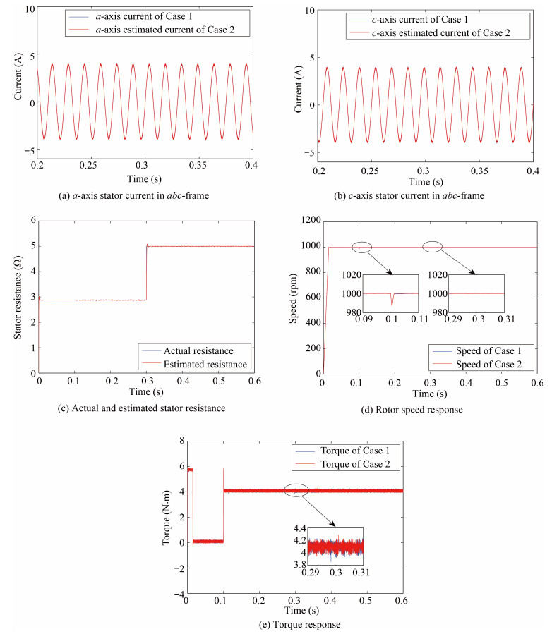
Fig. 4 Dynamic response comparison between Case 1 and Case 2 under the variation of stator resistance.

下载: 全尺寸图片幻灯片

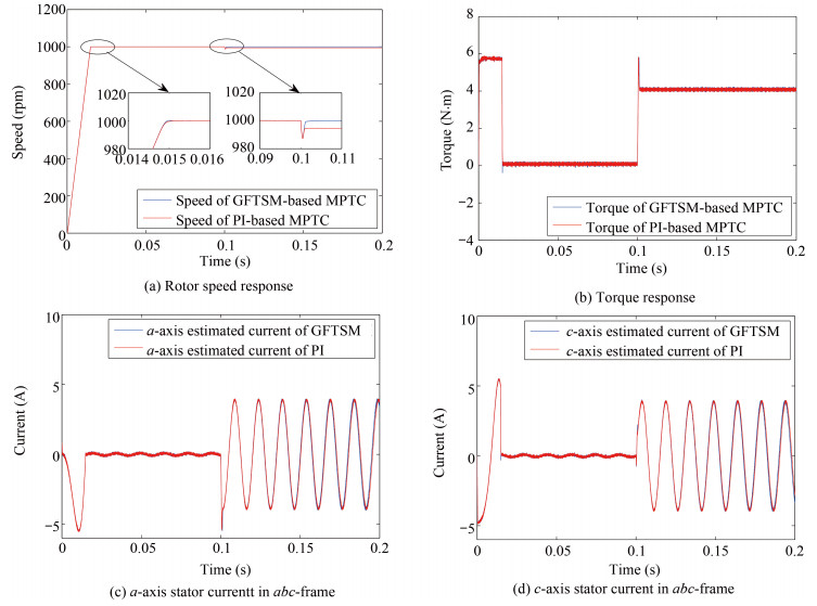
Fig. 5 The comparison of anti-load variation ability under the same speed transient response.

下载: 全尺寸图片幻灯片

Fig. 6 The comparison of dynamical response under the same speed anti-load variation ability.

下载: 全尺寸图片幻灯片

Fig. 7 The comparison of anti-load variation ability under the same speed transient response.

下载: 全尺寸图片幻灯片

Fig. 8 The comparison of dynamic response under the same anti-load variation ability.

下载: 全尺寸图片幻灯片

Table Ⅰ PARAMETERS OF PMSM DRIVE

Symbol	Value	Symbol	Value
$R_{\rm s}$	$2.875\, \Omega$	$\omega_{\rm r}^{\ast}$	1000 rpm
$L_{\rm d}, L_{\rm q}$	0.0085 H	$T_{\rm n}$	4 N$\cdot$m
$\psi_{\rm m}$	0.175 Wb	$J$	$0.0008\, {\rm Kg\cdot m}^2$
$p$	4	$B_{\rm m}$	0.001 N$\cdot$m$\cdot$s
$V_{\rm dc}$	300 V	$T_{\rm f}$	0

下载: 导出CSV

Table Ⅱ THD OF THREE-PHASE STATORS' CURRENT(%)

Control scheme	$i_{\rm a}$	$i_{\rm b}$	$i_{\rm c}$
PI-based MPTC	$2.21$	$2.32$	$2.24$
GFTSM-based MPTC	$1.84$	$1.88$	$1.85$

下载: 导出CSV

Table Ⅲ THD OF THREE-PHASE STATORS' CURRENT(%)

Control scheme	$i_{\rm a}$	$i_{\rm b}$	$i_{\rm c}$
SM-based MPTC	$2.01$	$2.12$	$2.14$
GFTSM-based MPTC	$1.84$	$1.88$	$1.85$

下载: 导出CSV

参考文献(36)

[1]	D. W. Chung and S. K. Sul, "Analysis and compensation of current measurement error in vector-controlled AC motor drives, "IEEE Trans. Ind. Appl. , vol. 34, no. 2, pp. 340-345, Mar. /Apr. 1998. http://ieeexplore.ieee.org/xpls/abs_all.jsp?arnumber=663477
[2]	Y. S. Jeong, S. K. Sul, S. E. Schulz, and N. R. Patel, "Fault detection and fault-tolerant control of interior permanent-magnet motor drive system for electric vehicle, "IEEE Trans. Ind. Appl. , vol. 41, no. 1, pp. 46-51, Jan. -Feb. 2005.
[3]	J. T. Boys, "Novel current sensor for PWM ac drives, "IEE Proc. Electr. Power Appl. , vol. 135, no. 1, pp. 27-32, Jan. 1988. http://ieeexplore.ieee.org/xpls/abs_all.jsp?arnumber=7636
[4]	H. Y. Ma, K. Sun, Q. Wei, and L. P. Huang, "Phase current reconstruction for AC motor adjustable-speed drives in the over-modulation method, "J. Tsinghua Univ. (Sci. Tech. ), vol. 50, no. 11, pp. 1751-1761, Nov. 2010. http://en.cnki.com.cn/Article_en/CJFDTOTAL-QHXB201011000.htm
[5]	T. C. Green and B. W. Williams, "Derivation of motor line-current waveforms from the DC-link current of an inverter, "IEE Proc. B: Electr. Power Appl. , vol. 136, no. 4, pp. 196-204, Jul. 1989. http://ieeexplore.ieee.org/xpls/abs_all.jsp?arnumber=32322
[6]	H. Kim and T. M. Jahns, "Phase current reconstruction for AC motor drives using a DC link single current sensor and measurement voltage vectors, "IEEE Trans. Power Electron. , vol. 21, no. 5, pp. 1413-1419, Sep. 2006. http://ieeexplore.ieee.org/xpls/icp.jsp?arnumber=1581804
[7]	J. I. Ha, "Current prediction in vector-controlled PWM inverters using single DC-Link current sensor, "IEEE Trans. Ind. Electron. , vol. 57, no. 2, pp. 716-726, Feb. 2010. http://ieeexplore.ieee.org/document/5196775/
[8]	K. Sun, Q. Wei, L. P. Huang, and K. Matsuse, "An over modulation method for PWM-inverter-fed IPMSM drive with single current sensor, "IEEE Trans. Ind. Electron. , vol. 57, no. 10, pp. 3395-3404, Oct. 2010. http://ieeexplore.ieee.org/document/5371830/
[9]	Y. K. Gu, F. L. Wei, D. P. Yang, and H. Liu, "Switching-state phase shift method for three-phase-current reconstruction with a single DC-Link current sensor, "IEEE Trans. Ind. Electron. , vol. 58, no. 11, pp. 5186-5194, Nov. 2011. http://ieeexplore.ieee.org/document/5727948/
[10]	B. Metidji, N. Taib, L. Baghli, T. Rekioua, and S. Bacha, "Low-cost direct torque control algorithm for induction motor without AC phase current sensors, "IEEE Trans. Power Electron. , vol. 27, no. 9, pp. 4132-4139, Sep. 2012. http://ieeexplore.ieee.org/document/6176236/
[11]	Y. S. Lai, Y. K. Lin, and C. W. Chen, "New hybrid pulse width modulation technique to reduce current distortion and extend current reconstruction range for a three-phase inverter using only DC-link sensor, "IEEE Trans. Power Electron. , vol. 28, no. 3, pp. 1331-1337, Mar. 2013. http://ieeexplore.ieee.org/document/6236197/
[12]	H. F. Lui, X. M. Chen, W. L. Qu, S. Sheng, Y. T. Li, and Z. Y. Wang, "A three-phase current reconstruction technique using single DC current sensor based on TSPWM, "IEEE Trans. Power Electron. , vol. 29, no. 3, pp. 1542-1550, Mar. 2014. http://ieeexplore.ieee.org/document/6531682/
[13]	Y. K. Gu, F. L. Ni, D. P. Yang, J. Dang, and H. Liu, "Novel method for phase current reconstruction using a single DC-link current sensor, "Electr. Mach. Contr. , vol. 13, no. 6, pp. 811-816, Dec. 2009. http://en.cnki.com.cn/Article_en/CJFDTOTAL-DJKZ200906006.htm
[14]	M. Carpaneto, P. Fazio, M. Marchesoni, and G. Parodi, "Dynamic performance evaluation of sensorless permanent-magnet synchronous motor drives with reduced current sensors, "IEEE Trans. Ind. Electron. , vol. 59, no. 12, pp. 4579-4589, Dec. 2012. http://ieeexplore.ieee.org/document/6134659/
[15]	Y. Cho, T. LaBella, and J. S. Lai, "A three-phase current reconstruction strategy with online current offset compensation using a single current sensor, "IEEE Trans. Ind. Electron. , vol. 59, no. 7, pp. 2924-2933, Jul. 2012. http://ieeexplore.ieee.org/document/6041024/
[16]	V. Verma, C. Chakraborty, S. Maiti, and Y. Hori, "Speed sensorless vector controlled induction motor drive using single current sensor, "IEEE Trans. Energy Convers. , vol. 28, no. 4, pp. 938-950, Dec. 2013. http://ieeexplore.ieee.org/document/6582551/
[17]	S. Morimoto, M. Sanada, and Y. Takeda, "High-performance current-sensorless drive for PMSM and SynRM with only low-resolution position sensor, "IEEE Trans. Ind. Appl. , vol. 39, no. 3, pp. 792-801, Mar. -Jun. 2003. http://ieeexplore.ieee.org/xpls/icp.jsp?arnumber=1201548
[18]	F. R. Salmasi and T. A. Najafabadi, "An adaptive observer with online rotor and stator resistance estimation for induction motors with one phase current sensor, "IEEE Trans. Energy Convers. , vol. 26, no. 3, pp. 959-966, Sep. 2011. http://ieeexplore.ieee.org/document/5953497/
[19]	Q. F. Teng, J. Y. Bai, J. G. Zhu, and Y. G. Guo, "Current sensorless model predictive torque control based on adaptive backstepping observer for PMSM drives, "WSEAS Trans. Syst. , vol. 13, no. 1 pp. 187-202, Jan. 2014. http://connection.ebscohost.com/c/articles/97265539/current-sensorless-model-predictive-torque-control-based-adaptive-backstepping-observer-pmsm-drives
[20]	J. Y. Yao, Z. X. Jiao, and D. W. Ma, "Adaptive robust control of DC motors with extended state observer, "IEEE Trans. Ind. Electron. , vol. 61, no. 7, pp. 3630-3637, Jul. 2014. http://ieeexplore.ieee.org/document/6594810/
[21]	W. C. Sun, Z. L. Zhao, and H. J. Gao, "Saturated adaptive robust control for active suspension systems, "IEEE Trans. Ind. Electron. , vol. 60, no. 9, pp. 3889-3896, Sep. 2013. http://ieeexplore.ieee.org/document/6226864/
[22]	S. Kouro, P. Cortes, R. Vargas, U. Ammann, and J. Rodriguez, "Model predictive control-A simple and powerful method to control power converters, "IEEE Trans. Ind. Electron. , vol. 56, no. 6, pp. 1826-1838, Jun. 2009. http://cpfd.cnki.com.cn/Article/CPFDTOTAL-ZGDN200905001474.htm
[23]	H. Miranda, P. Cortes, J. I. Yuz, and J. Rodriguez, "Predictive torque control of induction machines based on state-space models, "IEEE Trans. Ind. Electron. , vol. 56, no. 6, pp. 1916-1924, Jun. 2009. http://ieeexplore.ieee.org/document/4785128/
[24]	M. Preindl and S. Bolognani, "Model predictive direct torque control with finite control set for PMSM drive systems, Part 2: Field weakening operation, "IEEE Trans. Ind. Informat., vol.9, no.2, pp.648-657, May2013. doi: 10.1109/TII.2012.2220353
[25]	R. P. Aguilera, P. Lezana, and D. E. Quevedo, "Finite-control-set model predictive control with improved steady-state performance, "IEEE Trans. Ind. Informat., vol.9, no. 2, pp.658-667, May2013. doi: 10.1109/TII.2012.2211027
[26]	T. Geyer, G. Papafotiou, and M. Morari, "Model predictive direct torque control-Part Ⅰ: Concept, algorithm, and analysis, "IEEE Trans. Ind. Electron. , vol. 56, no. 6, pp. 1894-1905, Jun. 2009. http://ieeexplore.ieee.org/document/4663721/
[27]	C. E. García, D. M. Prett, and M. Morari, "Model predictive control: Theory and practice-A survey, "Automatica, vol.25, no.3, pp.335-348, May1989. doi: 10.1016/0005-1098(89)90002-2
[28]	Q. F. Teng, J. Y. Bai, J. G. Zhu, and Y. X. Sun, "Fault tolerant model predictive control of three-phase permanent magnet synchronous motors, "WSEAS Trans. Syst. , vol. 12, no. 8, pp. 385-397, Aug. 2013.
[29]	Q. F. Teng, J. Y. Bai, J. G. Zhu, and Y. G. Guo, "Sensorless model predictive torque control using sliding-mode model reference adaptive system observer for permanent magnet synchronous motor drive systems, "Control Theory Appl. , vol. 32, no. 2, pp. 150-161, Feb. 2015. http://en.cnki.com.cn/Article_en/CJFDTotal-KZLY201502003.htm
[30]	J. T. Gai, S. D. Huang, Q. Huang, M. Q. Li, H. Wang, D. R. Luo, X. Wu, and W. Liao, "A new fuzzy active-disturbance rejection controller applied in PMSM position servo system, "in Proc. 17th Int. Conf. Electrical Machines and Systems (ICEMS), Hangzhou, China, 2014, pp. 2055-2059. http://ieeexplore.ieee.org/xpls/abs_all.jsp?arnumber=7013842
[31]	X. G. Zhang, L. Z. Sun, K. Zhao, and L. Sun, "Nonlinear speed control for PMSM system using sliding-mode control and disturbance compensation techniques, "IEEE Trans. Power Electron. , vol. 28, no. 3, pp. 1358-1365, Mar. 2013. http://ieeexplore.ieee.org/document/6236202/
[32]	Q. F. Teng, G. F. Li, J. G. Zhu, and Y. G. Guo, "Sensorless active disturbance rejection model predictive torque control using extended state observer for permanent magnet synchronous motors fed by three-phase four-switch inverter, "Control Theory Appl., vol.33, no.5, pp.676-684, May2016.
[33]	J. Y. Yao, Z. X. Jiao, and D. W. Ma, "Extended-state-observer-based output feedback nonlinear robust control of hydraulic systems with backstepping, "IEEE Trans. Ind. Electron. , vol. 61, no. 11, pp. 6285-6293, Nov. 2014. http://ieeexplore.ieee.org/xpls/icp.jsp?arnumber=6733341
[34]	W. C. Sun, H. H. Pan, and H. J. Gao, "Filter-based adaptive vibration control for active vehicle suspensions with electrohydraulic actuators, "IEEE Trans. Veh. Technol. , vol. 65, no. 6, pp. 4619-4626, Jun. 2016. http://ieeexplore.ieee.org/document/7112535/
[35]	S. H. Yu, X. H. Yu, and Z. H. Man, "Robust global terminal sliding mode control of SISO nonlinear uncertain systems, "in Proc. 39th IEEE Conf. Decision and Control, Sydney, Australia, vol. 3, pp. 2198-2203, Dec. 2000. http://ieeexplore.ieee.org/xpls/abs_all.jsp?arnumber=914122
[36]	X. H. Yu and Z. H. Man, "Fast terminal sliding-mode control design for nonlinear dynamical systems, "IEEE Trans. Circuits Syst. Ⅰ: Fundam. Theory Appl. , vol. 49, no. 2, pp. 261-264, Feb. 2002. http://ieeexplore.ieee.org/xpls/icp.jsp?arnumber=983876