

-
摘要: 测试数据集的生成是软件组合测试的一个关键问题.为了提高测试数据的生成质量,提出了一种通过类搜索过程驱动的全局优化机制.在这个方法中,一个二进制编码机制被用于将组合测试数据生成问题转换为一个二进制基因序列的优化问题.同时,为了有效求解此问题,设计了一种新颖的全局优化算法—类搜索算法.此文主要论述了优化问题转换机制的可行性和有效性,并介绍了类搜索算法的计算机制.通过大量的仿真实验显示所提出的方法是可行的,且针对小规模组合测试问题,它是一种更为高效的组合测试数据集生成方法.
-
关键词:
- 类搜索算法(CSA) /
- 组合测试 /
- 全局优化 /
- 测试数据集优化
Abstract: The test suite generation is a key task for combinatorial testing of software. In order to generate high-quality testing data, a cluster searching driven global optimization mechanism is proposed. In this approach, a binary encoding mechanism is used to transform the combination test suite generating problem into a gene sequence optimization problem. Meanwhile, a novel global optimization algorithm, cluster searching algorithm (CSA), is developed to solve it. In this paper, the validity and rationality of problem transformation mechanism is verified, and the details of CSA are shown. The simulations illustrate the proposed mechanism is feasible. Moreover, it is a simpler and more efficient test suite generation approach for small-size combinatorial testing problems.-
Key words:
- Cluster searching algorithm (CSA) /
- combination test /
- global optimization /
- test suite optimization
-
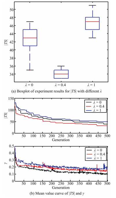
Fig. 5 Experiment statistical data for $CA(33;3, 6, 3)$ with different parameter $\lambda$.
Table Ⅰ A SUT WITH THREE TEST PARAMETERS
Value $A$ $B$ $C$ 0 a0 b0 c0 1 a1 b1 c1 2 a2 b2 c2  下载: 导出CSV
Table Ⅱ AN OPTIMAL TEST SUITE COVERING ALL PAIRWISE COMBINATIONS
Number $A$ $B$ $C $ 1 a0 b0 c0 2 a0 b2 c2 3 a0 b1 c1 4 a1 b0 c2 5 a1 b1 c0 6 a1 b2 c1 7 a2 b0 c1 8 a2 b2 c0 9 a2 b1 c2
下载: 导出CSV
Table Ⅲ AN ORDERLY COMPLETE TEST CASES SET
$A$ $B$ $C$ $t_j$ id $j$ a0 b0 c0 $t_0$ 0 a0 b0 c1 $t_1$ 1 a0 b0 c2 $t_2$ 2 a0 b1 c0 $t_3$ 3 $\vdots $ $\vdots $ $\vdots $ $\vdots $ $\vdots $ a2 b2 c2 $t_{26}$ 26
下载: 导出CSV
Algorithm 1 Decoding Input: positive integer $k$ and $v$, binary code of $I_i$ Output:test suite TS 1: for $j$ from 0 to $L-1$do 2: if $\alpha_j$ equal to 1 then 3: $dnum=j$; 4: for $m$ from 0 to $k-1$ do 5: $x = dnum$%$v; ~ dnum/=v$; 6: $t_j[m]=x$; 7: end for 8: put $t_j$ into TS; 9: end if 10:end for
下载: 导出CSV
Algorithm 2 Searching among group Input: population $Pop^{k-1}$ and cluster $C^{k-1}$ Output:$n$ offspring individuals in $Ch^k$ 1: Randomly select two different groups $C_i$ and $C_j$ ($i\neq j$) from current cluster $C^{k-1}$, then randomly select member $A_i^r$ and $A_j^s$ from $C_i$ and $C_j$ respectively. 2: Perform $\oplus$ operation between $A_i^r$ and $A_j^s$ to generate binary string $ch_1$ and $ch_2$. Then, perform $\odot$ operation on $ch_1$ and $ch_2$, respectively. That is $\begin{align}\begin{matrix} c{{h}_{1}},c{{h}_{2}}=\odot (A_{i}^{r}\oplus A_{j}^{s}). & (11) \\ \end{matrix}\end{align}$ 3: The number of offspring individuals $p=p+2$. If $p<n$, return to step 1. Otherwise, exit.
下载: 导出CSV
Algorithm 3 Searching among group Input: population $Pop^{k-1}$ and offspring individuals $Ch^k$ Output: new cluster $C^k$ 1: Set each $I_i$ in population to be a temporary group $C_i$. Initialize the IDM by (14). After that initialize the GDM by (15) based on IDM. Then, calculate the population diversity $\gamma$ by (13), and set the average group distance $\xi=\gamma$. 2: Find the minimum group distance $gdm_{pq}$ in GDM and merge the group $C_p$ and $C_q$ into a new group $C_{pq}$. Then, update the GDM. 3: Calculate new average group distance $\xi'$ $ \begin{align}\begin{matrix} {\xi }'=\frac{2}{|C|(|C|-1)}\sum\limits_{i=2}^{|C|}{\sum\limits_{j=1}^{i-1}{g}}d{{m}_{ij}} & (16) \\ \end{matrix} \end{align}$ where $|C|$ is the number of groups after step 2. If $\xi'<\xi$, go to step 4; otherwise, $\xi=\xi'$ and return step 2. 4: Restore the group $C_p$, $C_q$ and GDM. After that, update the center member for each group and output $C$.
下载: 导出CSV
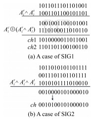
Algorithm 4 Searching inside group Input: $Pop^{k-1}$, $Ch^k$, $C^k$ and $\lambda$ Output: $m|C|$ offspring individuals in $Ch^k$ 1: Run this operation for $C_i$, $i=1, 2, \ldots, |C|$, and set $t=0$. 2: $UR(0, 1)$ is a uniformly distributed random number between 0 and 1. If $UR(0, 1)<\lambda$, goto step 2.1 to execute SIG1. Otherwise, goto step 2.2 to execute SIG2. 2.1: SIG1: select two members $A_i^r$ and $A_i^s$ from $C_i$ randomly, and execute logic and operation $\wedge$ between them. After that, perform multi-point crossover operation $\oplus$ between the output string by $A_i^r\wedge A_i^s$ and the center members $A_i^c$. This process can be expressed as $\begin{align}\begin{matrix} c{{h}_{1}},c{{h}_{2}}=A_{i}^{c}\oplus (A_{i}^{r}\wedge A_{i}^{s}). & (18) \\ \end{matrix}\end{align}$ After that, put the generating individuals $ch_1$ and $ch_2$ into $C_i$, $t=t+2$ and goto step 3. 2.2: SIG2: Randomly select three members $A_i^r$, $A_i^s$ and $A_i^t$ from $C_i$. Then, perform logic and operation $\wedge$ among them and output a binary string $ch$ $\begin{align}\begin{matrix} ch=A_{i}^{r}\wedge A_{i}^{s}\wedge A_{i}^{t}. & (19) \\ \end{matrix}\end{align}$ If $ch$ can cover all strength-$t$ combinations in CS, goto step 2.2.1. Otherwise, goto step 2.2.2. 2.2.1: Randomly select a valuable gene in $ch$, whose value is 1, and change it into 0. If the updated $ch$ still can cover all strength-$t$ combinations in CS, repeat this step. Otherwise, recover the value of last chosen gene to 1 and goto step 2.2.3. 2.2.2: Randomly select a gene in $ch$, whose value is 0, and change its value into 1. Then repeat this step until $ch$ has covered all strength-$t$ combination in CS and goto step 2.2.3. 2.2.3: Make the generating individuals $ch$ join $C_i$, set $t=t+1$ and goto step 3. 3: If $t<m$, update the $A_i^c$ of $C_i$ and return to step 2. Otherwise, set $i=i+1$ and return to step 1.
下载: 导出CSV
Algorithm 5 Cluster selection Input: $Pop^{k-1}$, $Ch^k$, $C^k$ Output: $Pop^k$ 1: For each $C_i$, sort its members in descending order by their fitness. After that, set $i=1$, $k=1$, $j=1$. 2: Take member $A_i^k$ from $C_i$ to be a surviving individual $I_j$ and join next population. It can be expressed as $\begin{matrix} {{I}_{j}}=A_{i}^{k},\quad j=1,2,\ldots ,n & {} \\ i=j \%|C|+1,\quad k=\text{round}\left( \frac{\mathit{j}}{|\mathit{C}|} \right)+1. & (20) \\ \end{matrix}$ 3: If $j<n$, $j=j+1$ and return to step 2; otherwise, exit.
下载: 导出CSV
Table Ⅳ EXPERIMENT STATISTICAL RESULTS OF 3 ALGORITHMS FOR 16 CA PROBLEMS WITH STRENGTH-2
$v$ $k$ $|\Phi|$ $\mathit{N}$ GA/OTAT GA/BCGO CSA TCA HHH Integer program $|TS|$ Time (s) $|TS|$ Time (s) $|TS|$ Time (s) $|TS|$ $|TS|$ $|TS|$ Time (s) Best Ave. Best Ave. Best Ave. Best Ave. Best Ave. Best Ave. 2 5 32 6 7 7.7 5.97 6 6 0.27 6 6 0.36 6 6.5 - - 6 - 0.70 6 64 - 7 8.1 6.54 6 6.2 0.68 6 6 1.10 6 6.7 - - 6 - 16.57 7 128 - 7 8.4 10.89 6 9.4 1.43 6 6 1.99 6 7.3 - - 6 - 441.2 8 256 - 8 10.7 12.71 6 11.3 3.91 6 6 4.70 6 7.0 - - - - - 9 512 - 8 11.2 14.5 40 51.6 7.49 6 6 9.60 7 7.9 - - - - - 10 1024 - 8 12.9 25.3 60 70.8 19.5 6 8.4 23.1 7 8.2 - - - - - 11 2048 7 9 14.2 28.8 141 167 40.3 7 9.5 49.0 8 8.7 - - - - - 12 4096 - 9 16.7 32.9 196 228 112.4 20 33.9 145 8 8.8 - - - - - 3 4 81 9 9 10.6 8.8 9 9 1.29 9 9 1.70 9 9.6 9 9 9 - 0.08 5 243 11 11 12.8 17.2 11 17.2 3.73 11 11 5.31 11 11.3 11 11.35 13 - * 6 729 12 16 18.1 19.6 44 57.8 11.5 12 12 14.9 13 14.1 13 14.2 - - - 7 2187 - 19 21.7 36.9 157 165 39.1 12 16.9 50.2 13 14.5 14 15 - - - 8 6561 13 20 27.9 40.3 224 277 133 88 97.5 148 14 14.7 15 15.6 - - - 4 5 1024 16 21 29.5 68.1 56 71.5 22.4 16 16.9 25.6 18 19.8 - - - - - 6 4096 19 25 36.7 74.4 197 227 194 22 34.2 223 21 22.7 - - - - - 7 16384 21 28 40.9 93 320 342 417 116 135 508 24 25.2 - - - - -
下载: 导出CSV
Table Ⅴ EXPERIMENT STATISTICAL RESULTS OF TEST CASE NUMBER FOR 16 CA PROBLEMS WITH STRENGTH-3
$v$ $k$ $|\Phi|$ $\mathit{N}$ GA/OTAT GA/BCGO CSA TCA HHH $|TS|$ Time (s) $|TS|$ Time (s) $|TS|$ Time (s) $|TS|$ $|TS|$ Best Ave. Best Ave. Best Ave. Best Ave. Best Ave. 2 5 32 10 11 13.6 11.1 10 11.2 0.41 10 10 0.42 10 10.6 - - 6 64 - 13 14.2 17.6 10 12.6 1.29 10 10 1.34 10 10.7 - - 7 128 - 14 15.6 24.4 12 15.1 2.09 10 10 2.15 10 11.2 - - 8 256 - 17 19.8 31.8 15 19.6 5.22 10 10 5.62 11 12.0 - - 9 512 - 19 21.9 41.0 17 23.9 9.85 10 10 11.0 11 11.9 - - 10 1024 - 22 25.2 52.3 41 54.7 25.9 10 11.8 25.3 13 15.8 - - 11 2048 12 24 27.7 69.9 80 92.8 56.8 12 19.4 55.5 14 15.5 - - 12 4096 15 28 30.9 82.1 239 257 131 69 85.7 133 17 18.1 - - 3 4 81 27 29 34.2 68.1 27 27 1.62 27 27 1.91 27 28.9 27 29.45 5 243 - 30 36.1 71.3 27 34.2 3.93 27 27 5.53 29 31.6 39 41.25 6 729 33 36 42.5 80.5 55 62.9 15.5 33 35.5 15.4 34 36.1 33 39 7 2187 39 48 54.4 89.9 195 217 87.9 49 54.9 93.2 46 47.7 49 50.8 8 6561 42 54 58.9 99.6 251 275 145 156 170 157 51 52.2 52 53.65 4 5 1024 64 72 81 148 60 78.2 22.7 64 67.9 27.6 66 68.7 - - 6 4096 88 93 105 198 229 249 212 194 216 231 94 96.6 - - 7 16384 - 99 117 153 370 379 499 233 247 527 96 98.4 - -
下载: 导出CSV
-
[1] D. R. Kuhn and M. J. Reilly, "An investigation of the applicability of design of experiments to software testing, "in Proc. 27th Annual NASA Goddard/IEEE Software Engineering Workshop, Greenbelt, MD, USA, 2002, pp. 91-95. http://ieeexplore.ieee.org/xpls/icp.jsp?arnumber=1199454 [2] D. R. Kuhn, D. R. Wallace, and A. M. Gallo, "Software fault interactions and implications for software testing, "IEEE Trans. Softw. Eng. , vol. 30, no. 6, pp. 418-421, Jun. 2004. http://dl.acm.org/citation.cfm?id=998624 [3] J. F. Wang, C. A. Wei, and Y. L. Sheng, "Locating errors in combinatorial testing using set of possible faulty interactions, "Acta Electron. Sinica, vol. 42, no. 6, pp. 1173-1178, Jun. 2014. http://en.cnki.com.cn/Article_en/CJFDTotal-DZXU201406021.htm [4] J. Yan and J. Zhang, "Combinatorial testing: Principles and methods, "Chin. J. Softw. , vol. 20, no. 6, pp. 1393-1405, Jun. 2009. [5] G. Seroussi and N. H. Bshouty, "Vector sets for exhaustive testing of logic circuits, "IEEE Trans. Inform. Theory, vol. 34, no. 3, pp. 513-522, May1988. http://www.ams.org/mathscinet-getitem?mr=959633 [6] J. Yan and J. Zhang, "A backtracking search tool for constructing combinatorial test suites, "J. Syst. Softw. , vol. 81, no. 10, pp. 1681-1693, Oct. 2008. http://dl.acm.org/citation.cfm?id=1401379 [7] C. J. Colbourn, S. S. Martirosyan, G. L. Mullen, D. Shasha, G. B. Sherwood, and J. L. Yucas, "Products of mixed covering arrays of strength two, "J. Combinat. Des. , vol. 14, no. 2, pp. 124-138, Mar. 2006. doi: 10.1002/jcd.20065/pdf [8] M. Sosina and T. van Tran, "On t-covering arrays, "Des. Codes Cryptogr. , vol. 32, no. 1-3, pp. 323-339, May2004. http://dl.acm.org/citation.cfm?id=993165 [9] F. Kang, S. X. Han, S. Rodrigo, and J. J. Li, "System probabilistic stability analysis of soil slopes using Gaussian process regression with Latin hypercube sampling, "Comput. Geotechn. , vol. 63, pp. 13-25, Jan. 2015. http://www.sciencedirect.com/science/article/pii/S0266352X1400161X [10] F. Kang, J. S. Li, and J. J. Li, "System reliability analysis of slopes using least squares support vector machines with particle swarm optimization, "Neurocomputing, vol. 209, pp. 46-56, Oct. 2016. http://www.sciencedirect.com/science/article/pii/S0925231216305859 [11] F. Kang, Q. Xu, and J. J. Li, "Slope reliability analysis using surrogate models via new support vector machines with swarm intelligence, "Appl. Math. Model. , vol. 40, no. 11-12, pp. 6105-6120, Jun. 2016. http://www.sciencedirect.com/science/article/pii/S0307904X16300464 [12] F. Kang and J. J. Li, "Artificial bee colony algorithm optimized support vector regression for system reliability analysis of slopes, "J. Comput. Civil Eng., vol.30, no.3, pp.04015040, May2016. doi: 10.1061/(ASCE)CP.1943-5487.0000514 [13] R. J. Zha, D. P. Zhang, C. H. Nie, and B. W. Xu, "Test data generation algorithms of combinatorial testing and comparison based on cross-entropy and particle swarm optimization method, "Chin. J. Comput. , vol. 33, no. 10, pp. 1896-1908, Oct. 2010. http://en.cnki.com.cn/Article_en/CJFDTotal-JSJX201010013.htm [14] Y. L. Liang and C. H. Nie, "The optimization of configurable genetic algorithm for covering arrays generation, "Chin. J. Comput. , vol. 35, no. 7, pp. 1522-1538, Jul. 2012. http://en.cnki.com.cn/Article_en/CJFDTotal-JSJX201207016.htm [15] C. H. Nie and J. Jiang, "Optimization of configurable greedy algorithm for covering arrays generation, "Chin. J. Softw. , vol. 24, no. 7, pp. 1469-1483, Jul. 2013. http://en.cnki.com.cn/Article_en/CJFDTotal-RJXB201307006.htm [16] J. K. Lin, C. Luo, S. W. Cai, K. L. Su, D. Hao, and L. Zhang, "TCA: An efficient two-mode meta-heuristic algorithm for combinatorial test generation (T), "in Proc. 30th IEEE/ACM Int. Conf. Automated Software Engineering (ASE), Lincoln, NE, USA, 2015, pp. 494-505. http://dl.acm.org/citation.cfm?id=2916166 [17] K. Z. Zamli, B. Y. Alkazemi, and G. Kendall, "A tabu search hyper-heuristic strategy for t-way test suite generation, "Appl. Soft Comput. , vol. 44, pp. 57-74, Jul. 2016. http://dl.acm.org/citation.cfm?id=2936563 [18] J. Yan and J. Zhang, "Backtracking algorithms and search heuristics to generate test suites for combinatorial testing, "in Proc. 30th IEEE Annual Int. Computer Software and Applications Conf. , Chicago, IL, USA, 2006, pp. 385-394. http://ieeexplore.ieee.org/xpls/icp.jsp?arnumber=4020100 [19] A. W. Williams and R. L. Probert, "Formulation of the interaction test coverage problem as an integer program, "in Testing of Communicating Systems XIV, US: Springer, 2002, pp. 283-298. doi: 10.1007/978-0-387-35497-2_21 [20] M. B. Cohen, P. B. Gibbons, W. B. Mugridge, and C. J. Colbourn, "Constructing test suites for interaction testing, "in Proc. 25th Int. Conf. Software Engineering, Portland, OR, USA, 2003, pp. 38-48. http://dl.acm.org/citation.cfm?id=776822&CFID=431488427&CFTOKEN=46085464 [21] L. Wang and L. P. Li, "A coevolutionary differential evolution with harmony search for reliability redundancy optimization, "Expert Syst. Appl. , vol. 39, no. 5, pp. 5271-5278, Apr. 2012. http://www.sciencedirect.com/science/article/pii/S0957417411015429 [22] I. Ciornei and E. Kyriakides, "Hybrid ant colony-genetic algorithm (GAAPI) for global continuous optimization, "IEEE Trans. Syst. Man Cybern. -Part B, vol. 42, no. 1, pp. 234-245, Feb. 2012. [23] M. Chateauneuf and D. L. Kreher, "On the state of Strength-Three Covering Arrays, "J. Combin. Des., vol.10, no.4, pp.217-238, May2002. doi: 10.1002/(ISSN)1520-6610 [24] R. Gelbard, O. Goldman, and I. Spiegler, "Investigating diversity of clustering methods: An empirical comparison, "Data Knowl. Eng. , vol. 63, no. 1, pp. 155-166, Oct. 2007. http://www.sciencedirect.com/science/article/pii/S0169023X07000031 -

 下载:
下载:


图(5) / 表(10)
计量
- 文章访问数: 2137
- HTML全文浏览量: 249
- PDF下载量: 607
- 被引次数: 0
