Guaranteed Consensus Control of Mobile Sensor Networks With Partially Unknown Switching Probabilities
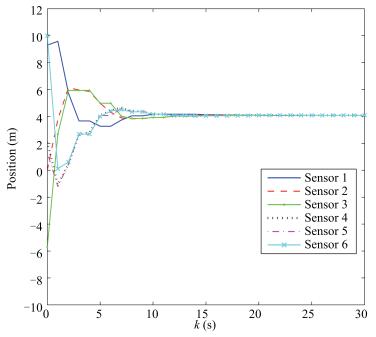
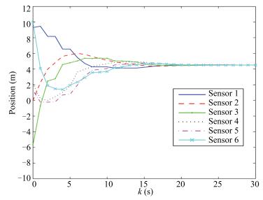
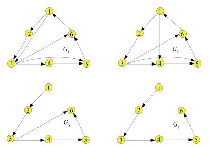
-
Abstract: This paper studies the guaranteed consensus of mobile sensor networks (MSNs) with stochastic switching topologies. The switching of topology is triggered by a Markov chain, whose initial and transition probabilities are partially unknown. Each topology in the switching topology set is a directed graph with a spanning tree. A set of distributed switching consensus controllers are derived by means of stability analysis of Markovian jump systems. This is achieved by defining a novel topology-aware cost function of the MSNs involving cost consumption for information receiving, sending and control. By state transformation, the initial dynamics of MSN is reduced to a Markovian jump system with guaranteed cost. A computational algorithm is proposed to simultaneously calculate both the sub-optimal controller gains and the sub-minimal upper cost bound. Eventually, the performance of the controller design method is verified by numerical examples.
-
Key words:
- Mobile sensor networks (MSNs) /
- Markov switching topologies /
- mean-square consensus /
- guaranteed cost control
-
1. Introduction
Mobile sensor networks (MSNs) have attracted increasing research attention and found various applications in the past decade [1], [2]. For a practical MSN, energy limitation is always one of the most important and challenging issues. The reason lies in the batteries powering the MSNs, which are limited in capacity and inconvenient for replacement. Besides, a typical MSN consists of a mass of energy-demanding nodes capable of sensing, computing, communicating and moving. As such, energy efficient algorithms are of utmost importance for MSN applications, hence, are the focus of many research works. To name a few, by modeling power consumption as the distance traveled by the sensors, [3]-[5] investigated the power-constrained deployment and coverage control issues of MSNs. In [6], an energy aware control protocol was proposed to achieve rendezvous without depleting the energy of the nodes. Based on the energy forecast, [7] designed a clustering-tree topology control algorithm to save energy and maximize the network lifetime for heterogeneous wireless sensor networks with considering packet loss rate and the link quality.
In most cases, the cost saving problem is complicated, since it is often realized at the cost of a certain degree of performance loss. Therefore, the intention of most papers comes down to finding a trade-off of energy usage and system performance, which refers to quality of performance (QoP) for control and estimation problems, and to quality of service (QoS) for communication problems. For instance, [8] investigated the compromise of communication cost and the convergence rate (a QoP indicator), and [9] studied the trade-off between energy expenditure and communication delay (a QoS parameter).
Here we aim at the issue of consensus seeking of MSNs subject to limited cost supply. Of course, it is not the first time that this problem is being addressed. There have been some results reported in the literature. For instance, [10] considered the energy-constrained consensus estimation issue by activating a subset of sensors at each instant. In [11], an optimal consensus controller design method was given to minimize the power cost of sensors deployed in smart home systems. Reference [12] proposed an LQR consensus algorithm for multi-vehicle control. In [13], a sub-optimal consensus control algorithm for MSNs was presented by modeling the energy expenditure for mobility and communication independently. Most of these results assume static communication topologies in the MSNs. In practice, however, the network topology may vary with link failures, packet dropouts or environmental disturbances. As these factors are random by nature, the switching of topologies is essentially a random event modeled as a stochastic process, in particular, a Markov chain [14]. In fact, a number of papers have studied MSNs with Markov switching topologies under different frameworks with various concerns, see, e.g., in [15]-[21]. However, it should be noted that several important factors have not been considered in the existing results. Firstly, most of these works concern ergodic Markov chains, while a more general Markov chain is more interesting, since when a system goes through an unsteady environment to a settled one, it will reasonably experience switching from variable topology to a certain fixed one. Secondly, almost all the existing results are applied to situations with completely known transition probabilities. In reality, however, all or part of the transition probabilities are unavailable [22]-[25], and only the estimated values of transition rates are accessible. Moreover, estimation errors, referred to as probability uncertainties of switching topology, may also result in instability or at least degrade performance of MSNs. Thus, it is of great importance to consider partially unavailable transition rates, which do not need any knowledge of the unavailable elements. Thirdly, existing works do not consider cost limitations.
In this paper, we study the guaranteed cost consensus seeking problem for MSNs with switching communication topologies governed by a Markov chain whose initial and transition probabilities are partially unknown. A team of mobile sensors cooperate with each other and form a network whose topologies are switching within a topology set according to a Markov chain. Each directed graph in the graph set is assumed to have a spanning tree. A novel function of team cost which penalizes the state and control input errors between communicating sensors is defined in a linear quadratic form, in which cost consumption for information receiving and sending is involved. The elements of the transition probability matrix are divided into the known and unknown parts. Then, using model transformation and graph theory, the issue of guaranteed cost consensus is transformed to the stability problem of a reduced order Markov jump systems with partially unknown initial and transition probabilities. Using stochastic Lyapunov functional method, a sufficient mean square stability condition is obtained for the reduced order jumping system, which guarantees global exponential consensus of the original MSN in the mean square sense. Then, a computational algorithm is given, by which the sub-optimal controller gains and a sub-minimal upper cost bound of the MSN can be calculated, concurrently. The validity of the controller design method is illustrated by example results.
The remaining sections are organized as follows. Section 2 provides some preliminaries of graph theory, Markov switching topology and the problem formulation. The main results on sufficient consensus condition are presented in Section 3. Then, a controller design algorithm of sensor networks is derived. In Section 4, numerical examples are given to validate the performance of the proposed method. Section 5 draws a conclusion.
Notations: $\mathbb{R}^{n }$ and $\mathbb{R}^{n\times m}$ denotes $n$ dimensional Euclidean space and the family of dimensional real matrices, respectively. $I_{n}$ stands for $n$ dimensional identity matrix. For a given matrix $X$ , $\| X \|$ denotes its Euclidean norm, $X^{T}$ denotes its transpose, and $X^{-1}$ denotes its inverse matrix (if square matrix $X$ is nonsingular). And ${\rm diag}\{\cdot\} $ denotes a block-diagonal matrix. The sign $\otimes $ represents Kronecker product of matrix. 0 denotes a column vector whose entries equal to zero. The similar notation is adopted for 1. ${\rm Pro}(y)$ and ${E}(y)$ denote the probability and mathematical expectation of stochastic variable $y$ . $\mathbb{N}^+$ denotes the non-negative integers. ∅ denotes an empty set which implies that there are no elements in the set according to some rules.
2. Preliminaries and Problem Statement
2.1 Graph Theory Notations
Consider a mobile sensor network consisting of $N$ identical sensors. A directed graph (digraph) is used to model the interactions among sensors, where $\upsilon \in \{\upsilon _1$ $\ldots$ $\upsilon _N \}$ is the set of $N$ nodes, $\varepsilon \subseteq \upsilon \times \upsilon $ is the set of edges, $\Lambda =[a_{ij}]$ is the adjacency matrix with its elements associated with the edges, i.e., if , $a_{ij}$ $=$ $1$ , otherwise $(\upsilon _i, \upsilon _j)\notin \varepsilon $ , $a_{ij}=0$ . Edge $(\upsilon _i, \upsilon _j)\in \varepsilon $ means that node $\upsilon _i $ can receive information transmitted from node $\upsilon _j $ . A sequence of edges $(\upsilon _i, \upsilon _k)$ , $(\upsilon _k, \upsilon _l)$ , $\ldots $ , is called a directed path from node $\upsilon _j $ to node $\upsilon _i $ . A digraph is said to have a spanning tree, if there is a directed path from the root to any other nodes in the graph. The set of in-neighbors of node $\upsilon _i $ at time $k$ is denoted by . Similarly, the set of out-neighbors of node $\upsilon _i $ is adopted as $N_i^{\rm out} (k)$ $=$ . The in-degree of node $\upsilon _i $ is defined as $d_i =\sum\nolimits_{j=1}^N {a_{ij} } $ , moreover, in-degree matrix $\Delta ={\rm diag}\{d_1, \ldots, d_N \}$ . The Laplacian matrix of the directed graph $G$ is defined as $L=\Delta -\Lambda $ . Accordingly, the out-degree of node $\upsilon _i $ is defined as $d_i ^o=\sum\nolimits_{j=1}^N {a_{ji} } $ and the out-degree matrix $\Delta ^o={\rm diag}\{d_1 ^o, \ldots, d_N ^o\}$ . The column Laplacian matrix of graph $G$ is defined as .
2.2 Markov Switching Topology With Partially Unknown Switching Probabilities
At each instant $k$ , the interconnection of these mobile sensors can be regarded as a directed graph with a spanning tree. The communication topology is not fixed but switching according to a certain random event. It is assumed that the topology is switching within a given set of graphs $G( {\theta (k)})\in\bar {G}(k)$ , , where $k$ $\in$ $\mathbb{N}^+\}$ is the switching signal. Here, $\{\theta (k), k\in \mathbb{N}^+\}$ is assumed to be a Markov chain taking values in a finite set, $\theta (k)$ $\in$ , with transition probability defined as
$ \begin{align*} {\rm Pro}\{\left. {\theta (k+1)=v} \right|\theta (k)=l\}=\pi _{lv} \end{align*} $
where ${\rm Pro}\{\theta(0)=l\}=\pi_{0 l} $ , $\pi _{0l} $ is the initial probability of $G_{l}$ , $\forall l\in S$ , is the initial probability distribution, $\pi _{lv} $ is the single step transition probability from mode $l$ to mode $v$ , $\sum_{v=1}^q {\pi _{lv} =1} $ , , $\pi =[\pi _{lv}]_{q\times q} $ is called transition probability matrix.
The transition probabilities of the Markov chain are assumed to be partly available, e.g., some elements in transition probability matrix $\pi $ are unknown. For example, when $q$ $=$ $4, $ the transition probability matrix $\pi $ may be
$ \begin{align*} \pi =[\pi _{lv}]_{4\times 4} =\left[{{\begin{array}{*{20}c} {\pi _{11} } \hfill & {\pi _{12} } \hfill & ? \hfill & ? \hfill \\ ? \hfill & ? \hfill & {\pi _{23} } \hfill & ? \hfill \\ {\pi _{31} } \hfill & ? \hfill & {\pi _{33} } \hfill & ? \hfill \\ {\pi _{41} } \hfill & {\pi _{42} } \hfill & {\pi _{43} } \hfill & {\pi _{44} } \hfill \\ \end{array} }} \right] \end{align*} $
where ? represents the unavailable element. Define $S=$ $\cup$ $S_{u\kappa }^l $ , where $S_\kappa ^l ={\{}v, $ if is known}, $S_{u\kappa }^l ={\{}v, $ if $\pi _{lv} $ is unknown} for any $l\in S$ . The former is equivalently described as $S_\kappa ^l =\{\kappa _1^l, \ldots, \kappa _r^l \}$ , , where $\kappa _r^l$ $\in$ $\mathbb{N}^+$ represents the $r$ {th} known element in the $l$ {th} row of matrix $\pi $ . In the forthcoming discussions, notation $\pi _\kappa ^l=$ will be adopted. Furthermore, the initial probability distribution is also assumed partially unknown, i.e., $\Pi _0$ $ =$ , we denote $\Omega _\kappa = \{v$ , if is known}, $\Omega _{u\kappa } =\{v$ , if $\pi _{0v} $ is unknown}, $1\le v\le q$ . Also, we denote throughout the paper.
2.3 Problem Statement and the Control Objective
The dynamics of each sensor in the MSN is presented as:
$ \begin{align}\label{system} x_i (k+1)=Ax_i (k)+Bu_i (k), \quad i=1, {\ldots}, N \end{align} $
(1) where $x_i (k)\in \mathbb{R}^n$ and $u_i (k)\in \mathbb{R}^m$ are the state and control input of sensor $i$ , and $B\in \mathbb{R}^{n\times m}$ are constant matrices, $x_i (0)$ is the initial state.
As in many other references [26], it is assumed that a number of mobile base stations are deployed to detect the topology information of the MSN and broadcast the information of the communication topology to the sensors in the systems, which implies it is a practical way that each sensor can know the present topology. Therefore, we use the mode-dependent consensus control protocol for sensor as follows.
$ \begin{align}\label{eq1} u_i \mbox{(}k\mbox{)}=K(\theta (k))\sum\limits_{j\in N_j } {a_{ij} (\theta (k))(x_i(k)-x_j (k))}, \quad \theta (k)\in S \end{align} $
(2) where $K(\theta (k))$ is the controller gain matrix to be designed later.
The cost consumption for information receiving, sending and control of the MSN (1), respectively, can be defined as below
$\begin{align} \label{eq2} & C_r =\sum\limits_{k=0}^{\infty} {\sum\limits_{i=1}^N {{E}\left( {z_i^T (k)Q_1 z_i (k)} \right)} } \end{align} $
(3) $ \begin{align} \label{eq3} & C_s =\sum\limits_{k=0}^{\infty}{\sum\limits_{i=1}^N {{E}\left( {y_i^T (k)Q_2 y_i (k)} \right)} } \end{align} $
(4) $ \begin{align} \label{eq4} & C_c =\sum\limits_{k=0}^{\infty} {\sum\limits_{i=1}^N {{ E}\left( {u_i^T (k)Ru_i (k)} \right)} } \end{align} $
(5) where , , $R\in \mathbb{R}^{m\times m}>0$ and $Q_1, $ are constant matrices.
Remark 1: In many wireless sensor network applications, data transmitting and receiving are two different procedures with different power requirement. This paper gives independent considerations of the energy costs for information receiving and sending. To cope with them more accurately, we use the to describe sensors from which sensor i receives information at each sampling instant, and $j$ $\in$ $N_i^{\rm out} (k)$ to denote sensors to which senor $i$ transmits information. We also introduce weight matrices $Q_1$ and $Q_2$ in the cost function to make independent penalties on the two cost consumption procedures. Therefore, the method proposed in this paper is very flexible for use in different scenarios.
The objective of this paper is to design a set of controllers (2) for MSN (1) to achieve consensus in the sense defined below.
Definition 1: MSN (1) is said to achieve mean-square consensus (MS-consensus) with consensus protocol (2) under Markov switching topologies $G( {\theta (k)} )$ , , $\theta (k)$ $\in$ $S=\{1, \ldots, q\}$ , if for any initial $x_i (0)$ , the following
$ \begin{align*} \lim\limits_{k\to \infty } {E}\left[{\left\| {x_i (k)-x_j (k)} \right\|^2} \right]=0 \end{align*} $
holds true for any $i, $ $j=1, {\ldots}, N.$ Furthermore, the consensus protocols should guarantee a limited cost consumption:
$ \begin{align} \label{eq5} C= & \sum\limits_{k=0}^\infty \sum\limits_{i=1}^N {\rm e}\left( z_i^T (k)Q_1 z_i (k)+\right. \left.y_i^T (k)Q_2 y_i (k) \right.\nonumber\\ & \left.+u_i^T (k)Ru_i (k) \right) . \end{align} $
(6) Specifically, we aim at designing controllers (2) such that MSNs achieve consensus seeking for $C\le \tilde {C}$ , where is a given cost budget.
3. Main Results
In this section, firstly, the sufficient MS-consensus conditions for MSN (1) with partially unknown switching probabilities will be derived. Then, using this condition, a controller design algorithm will be given to simultaneously calculate controller gains and sub-minimal cost upper bound.
Let $I_k =\{x\left( t \right), \theta (t), t=0, 1, 2, \ldots, k\}$ be the admissible information set. Then, under the consensus protocol (2), the dynamics of MSN (1) can be rewritten as
$ \begin{equation} \label{eq6} X(k+1)=(I_N \otimes A+L_\theta \otimes BK_\theta )X(k) \end{equation} $
(7) where $X(k)=[x_1^T (k), x_2^T (k), \ldots, x_N^T (k)]^T$ , Laplacian matrix $L_\theta$ $=$ $L(\theta (k))$ and the controller gain $K_\theta =K(\theta (k))$ .
By the definition of , $Y(k)=[y_1^T (k), y_2^T (k), \ldots, y_N^T (k)]^T$ , we can obtain $Z(k)=(L_\theta \otimes I_N)X(k)$ , , where $L_\theta ^o =L^o(\theta (k))$ . The global cost of the MSN (1) can be rewritten as
$ \begin{align} \label{eq7} C= & \ \sum\limits_{k=0}^\infty {E}\left( X^T(k)\left( \left( L_\theta ^T L_\theta \right)\otimes Q_1 +\left( (L_\theta^o)^TL_\theta^o \right)\otimes Q_2 \right.\right.\nonumber\\ & \left.\left.\ +\left( L_\theta^T L_\theta \right)\otimes K_\theta^T RK_\theta \right)X(k)\right) . \end{align} $
(8) Now, introduce the following state transformation [21]:
$ \begin{equation} \label{eq8} \tilde {X}(k)=(T\otimes I_n)^TX(k). \end{equation} $
(9) And partition $\tilde {X}(k)\in \mathbb{R}^{nN}$ into two parts as $\tilde {X}(k)=[\tilde {X}_1^T (k), $ $\tilde {X}_2^T (k)]^T$ , where $\tilde {X}_1 (k)\in \mathbb{R}^n$ is a vector consisting of the first $n$ elements of $\tilde {X}(k)$ . Then, the dynamics of system (7) can be written as
$ \begin{align} \label{eq9} \tilde {X}_1 (k+1)= & ~A\tilde {X}_1 (k)+\Theta _\theta \otimes BK_\theta \tilde {X}_2 (k) \end{align} $
(10) $ \begin{align} \label{eq10} \tilde {X}_2 (k+1)= & ~(I_{N-1} \otimes A+{\Phi} _\theta \otimes BK_\theta)\tilde {X}_2 (k) \end{align} $
(11) where $\Theta _\theta =\frac{1}{\sqrt N }1^TL_\theta T_o $ , . According to [21], the MS-consensus of MSN (1) will be achieved if system (11) is mean square stable. Also, the cost consumption (8) can be rewritten as follows
$ \begin{align} \label{eq11} C= & \ \sum\limits_{k=0}^\infty {E}\left( \tilde {X}_2^T(k)\left( ( {{\Phi}_\theta^T {\Phi}_\theta } )\otimes Q_1 \right.\right.\nonumber\\ & +( {({\Phi}_\theta^o) ^T{\Phi}_\theta^o } )\otimes Q_2 \notag\\ & \left.\left. + ( {{\Phi}_\theta^T {\Phi}_\theta } )\otimes K_\theta^T RK_\theta \right)\tilde {X}_2 (k)\right) \end{align} $
(12) where ${\Phi} _\theta ^o =T_o ^TL_\theta ^o T_o $ .
With the above discussion, the consensus seeking issue of system (7) is transformed to the stability problem of the reduced order system (11) with performance index (12).
We are now in the position to establish a sufficient mean square stability condition for system (11) with a guaranteed energy cost $\tilde {C}$ .
Theorem 1: Under the consensus protocol (2), MSN (1) can achieve guaranteed cost MS-consensus with Markov switching topologies set $\bar {G}(k)$ , if there exist matrices $P_l >0$ , $P_l$ $\in$ $R_{(N-1)n\times (N-1)n} $ , $l\in S$ , such that the following conditions
$ \begin{align} \label{eq12} \Psi _l^T & \sum\limits_{v\in S_\kappa ^l } {\pi _{lv} P_v } \Psi _l -\pi _\kappa ^l \Big(P_l -Q_l -Q_l^o \nonumber\\ & - (I_{N-1} \otimes K_l)^TR_l (I_{N-1} \otimes K_l) \Big)<0, \quad v\in S_\kappa ^l \end{align} $
(13) $ \begin{align} \Psi _l^T & P_v \Psi _l -P_l +Q_l +Q_l^o \nonumber\\ & +(I_{N-1} \otimes K_l)^TR_l (I_{N-1} \otimes K_l)<0\label{eq13}, \quad\ \ v\in S_{u\kappa }^l \end{align} $
(14) hold true, where , ${\Phi} _l =T_o ^TL_l T_o $ , $L_l$ $=L(\theta (k)=l)$ , , , ${\Phi}_l^o $ $=T_o ^TL_l^o T_o $ , , and $T_o $ is the orthogonal basis for the null space of 1. Furthermore, the guaranteed cost is
$ \begin{equation} \label{eq14} C\le \tilde {C}=\tilde {X}_2^T (0)\left( {\sum\limits_{v\in \Omega _\kappa } {\pi _{0v} } P_v +(1-\pi _\kappa ^0)\sum\limits_{v\in \Omega _{u\kappa } } {P_v } } \right)\tilde {X}_2 (0). \end{equation} $
(15) Proof: Firstly, the stability of system (11) will be proved. The following stochastic Lyapunov functional is defined as
$ \begin{equation} \label{eq15} V(k, \theta (k))=\tilde {X}_2^T (k)P_{\theta (k)} \tilde {X}_2 (k), \quad \theta (k)\in S=\{1, \ldots, q\}. \end{equation} $
(16) Let $\theta (k)=l$ , $\theta (k+1)=v$ , $l, v\in S$ , the backward difference of (16) is derived as
$ \begin{align} \Delta V(k)= & ~{E} (V(k+1, \left| {I_k } \right.)-V(k) \nonumber\\= & ~{E} (\tilde {X}_2^T (k+1)P_v \tilde {X}_2 (k+1)\left| {I_k } \right.)-\tilde {X}_2^T (k)P_l \tilde {X}_2 (k) \nonumber\\= & ~\tilde {X}_2^T (k)\left( {\Psi _l^T \sum\limits_{v\in s} {\pi _{lv} P_v } \Psi _l -P_l } \right)\tilde {X}_2 (k).\label{eq16} \end{align} $
(17) Since , (17) can be written as
$ \begin{align} \label{eq17} \Delta V(k)= & ~\tilde {X}_2^T (k)\left( \Psi _l^T \left( {\sum\limits_{v\in S_\kappa ^l } {\pi _{lv} P_v } +\sum\limits_{v\in S_{u\kappa }^l } {\pi _{lv} } P_v }\right)\Psi _l \right.\nonumber \\ & \left.-\left( {\sum\limits_{v\in S_\kappa ^l } {\pi _{lv} } +\sum\limits_{v\in S_{u\kappa }^l } {\pi _{lv} } } \right)P_l \right)\tilde {X}_2 (k). \end{align} $
(18) If (13) and (14) hold, we can have
$ \begin{align} \Psi _l^T & \sum\limits_{v\in S_\kappa ^l } {\pi _{lv} P_v } \Psi _l -\pi _\kappa ^l \Big( P_l -Q_l -Q_l^o \nonumber\\ & - (I_{N-1} \otimes K_l)^TR_l (I_{N-1} \otimes K_l) \Big) \nonumber\\ & +\sum\limits_{v\in S_{u\kappa }^l } \pi _{lv} \left( \Psi _l^T P_v \Psi _l -P_l +Q_l +Q_l^o \right. \nonumber\\ & \left.+ (I_{N-1} \otimes K_l)^TR_l (I_{N-1} \otimes K_l) \right) <0.\label{eq18} \end{align} $
(19) Employing (18) and (19), the difference satisfies
$ \begin{equation} \label{eq19} \Delta V(k)\le -\tilde {X}_2^T (k)F_l \tilde {X}_2 (k) \end{equation} $
(20) where . Based on (18) and (20), we can obtain that
$ \begin{align} {E} (V(k+1\left| {I_k } \right.) & \le V(k)-\tilde {X}_2^T (k)F_l \tilde {X}_2 (k)\nonumber\\ & \le \left( {1-\frac{\lambda _{\min } (F_l)}{\lambda _{\max } (P_l)}} \right)V(k)=\zeta V(k).\label{eq20} \end{align} $
(21) If inequalities (13) and (14) hold, it is clear that $<$ $\lambda _{\max } (P_l)$ , $0<\zeta <1$ . Along the same lines, the following formulation can be obtained
$ \begin{equation} \label{eq21} E(V(k)\left| {I_{k-1} } \right.)=\zeta V(k-1). \end{equation} $
(22) According to smooth characteristics of conditional mean [27], by (22), we can have
$ \begin{align} \label{eq22} {E} (V(k)\left| {I_{k-2} } \right.)= & ~{E} ({\rm e}(V(k)\left| {I_{k-1} } \right.)\left| {I_{k-2} } \right.)\nonumber\\\le & ~\zeta {E} (V(k-1)\left| {I_{k-2} } \right.)\nonumber\\\le & ~\zeta ^2V(k-2). \end{align} $
(23) By recursion like (21), (22) and (23), the exponentially mean square stable condition can be derived as
$ \begin{align} \label{eq23} {E} (V(k))= & ~{E} (\tilde {X}_2^T (k)P_{\theta (k)} \tilde {X}_2 (k))\nonumber\\\le & ~\zeta ^kV(0)=\zeta ^k\tilde {X}_2^T (0)P_{\theta (0)} \tilde {X}_2 (k) \end{align} $
(24) from which it is straightforward that
$ \begin{equation} \label{eq24} {E} (\tilde {X}_2^T (k)P_{\theta (k)} \tilde {X}_2 (k))\le \beta \zeta ^k\tilde {X}_2^T (0)\tilde {X}_2 (0) \end{equation} $
(25) where , $0<\zeta <1$ . Therefore, the stability of the reduced order system (11) can be achieved exponentially in a mean square sense. Moreover, under Markov switching topologies, the MSN (1) with controller (2) can achieve MS-consensus
Next, the proof of the guaranteed cost will be given. Summing both sides of inequality (17) from $k=0$ to $\infty$ yields
$ \begin{align} \label{eq25} C= & ~\sum\limits_{k=0}^\infty {{E} (\tilde {X}_2 ^T(k)F_u \tilde {X}_2 (k)})\nonumber\\\le & ~{E} \left( {V(0, \theta (0))} \right)\nonumber\\= & ~{E} (\tilde {X}_2^T (0)P_{\theta (0)} \tilde {X}_2 (0))=\tilde {J} \quad \forall l\in S. \end{align} $
(26) Since $\pi _{ov} \le 1-\pi _\kappa ^0 $ , , the energy cost upper bound in (26) can be written as
$ \begin{equation} \label{eq26} \tilde {C}=\tilde {X}_2^T (0)\left( {\sum\limits_{v\in \Omega _\kappa } {\pi _{0v} } P_v +(1-\pi _\kappa ^0)\sum\limits_{v\in \Omega _{u\kappa } } {P_v } } \right)\tilde {X}_2 (0). \end{equation} $
(27) Remark 2: If $S_{u\kappa }^l =∅$ , $\forall l\in S$ , the problem reduces to the case where the initial and transition probabilities of the Markov chain are completely known [28]. In this case, the conditions in (13) and (14) are simplified as , $l\in S$ . On the other hand, if $S_\kappa ^l = ∅$ , $\forall l\in S$ , then the problem reduces to the case with arbitrary switching topologies [29] and conditions (13) and (14) become as $Q_l$ $+$ , $l\in S$ .
Before closing this section, a design algorithm for the controllers (2) will be proposed. To derive the algorithm, the following sufficient conditions on the existence of the controller gains are needed.
Theorem 2: For MSN (1) under Markovian switching topologies $G(\theta (k))$ , the consensus protocols (2) can drive the MSN to reach guaranteed cost consensus, if there exist $P_l $ , $M_l \in \mathbb{R}^{(N-1)n\times (N-1)n}$ , , $M_l >0$ , such that the following conditions
$ \begin{align} \label{eq27} & \begin{bmatrix} {-\pi _\kappa ^l \left( {P_l -Q_l -Q_{l^o} } \right)} & {\sqrt {\pi _\kappa ^l } \left( {I_{N-1} \otimes K_l } \right)^T} & {\Psi _l^T } \\ {\sqrt {\pi _\kappa ^l } \left( {I_{N-1} \otimes K_l } \right)} & {-R_l^{-1} } & 0 \\ {\Psi _l } & 0 & {-M_l } \end{bmatrix}<0 \nonumber\\ & ~~~~~~~~~~~~~~~~~~~~~~~~~~~~~~~~~~~~~~~~~~~~~~~~~~~ v\in S_\kappa ^l \end{align} $
(28) $ \begin{align}& \label{eq28} \left[{{\begin{array}{*{20}c} {-P_l +Q_l +Q_{l^o} } & {\left( {I_{N-1} \otimes K_l } \right)^T} & {\Psi _l^T } \\ {\left( {I_{N-1} \otimes K_l } \right)} & {-R_l^{-1} } & 0 \\ {\Psi _l } & 0 & {-H_v } \\ \end{array} }} \right]<0 \nonumber\\ & ~~~~~~~~~~~~~~~~~~~~~~~~~~~~~~~~~~~~~~~~~~~~~~~~~~~ v\in S_{u\kappa }^l \end{align} $
(29) hold for all $l\in S$ , with the constraint and , $v\in S_{u\kappa }^l $ .
Proof: By using Theorem 1 and Schur complement lemma, Theorem 2 can be easily proved, so we omit it.
As for the cost budget of the MSNs, a feasible one has been derived in Theorem 1. Since the capacity of batteries for the MSNs is restricted, a minimal cost bound is more appropriate. Namely, we intend to seek the infimum of $\tilde {C}$ in (15) over the feasibility set $\Delta =(P_l, M_l, K_l)$ $(l\in S)$ determined by Theorem 2 as
$ \begin{align} \label{eq29} C^* & =\inf \limits_\Delta \tilde{C}\notag\\ & = \inf \limits_\Delta \tilde {X}_2^T (0)\left( \sum\limits_{v\in \Omega _\kappa } {\pi _{0v} } P_v +(1-\pi _\kappa ^0)\sum\limits_{v\in \Omega _{u\kappa } } {P_v } \right)\tilde {X}_2 (0). \end{align} $
(30) The minimization problem can be presented as
$ \begin{align} & {\min}~\delta \end{align} $
(31) $ \begin{align} & {\rm s. t.}~~\delta \ge \tilde {X}_2^T (0)\left( {\sum\limits_{v\in \Omega _\kappa } {\pi _{0v} } P_v +(1-\pi _\kappa ^0)\sum\limits_{v\in \Omega _{u\kappa } } {P_v } } \right)\tilde {X}_2 (0). \end{align} $
(32) By Schur complement, equivalently, it can be written as
$\begin{equation} \label{eq30} \left[{{\begin{array}{*{20}c} \delta & {\tilde {X}_2^T (0)} & {\tilde {X}_2^T (0)} \\ {\tilde {X}_2 (0)} & {M_{\Omega _\kappa }^0 } & 0 \\ {\tilde {X}_2 (0)} & 0 & {M_{\Omega _{u\kappa } }^0 } \\ \end{array} }} \right]\ge 0 \end{equation} $
(33) where
$ M_{\Omega _\kappa }^0 =\left( {\sum\limits_{v\in \Omega _\kappa } {\pi _{0v} P_v } } \right)^{-1} $
and
$ M_{\Omega _{u\kappa } }^0 =\left( {(1-\pi _\kappa ^0)\sum\limits_{v\in \Omega _{u\kappa } } {P_v } } \right)^{-1}. $
The conditions in (33), (28) and (29) contain some constraints of matrix inversion, which are equivalent to the rank constrained LMIs
$ \begin{align} & \left\{\begin{aligned}\label{eq34} & \varXi_v=\begin{bmatrix} \sum\limits_{v\in \Omega_\kappa } \pi_{0v} P_v & \ast \\ I & M_{\Omega_\kappa }^0 \end{bmatrix}\ge 0 \\ & {\rm Rank} (\varXi_v)\le (N-1)n, \quad v\in \Omega _k \end{aligned}\right. \end{align} $
(34) $ \begin{align} & \left\{\begin{aligned}\label{eq35} & \varXi_v=\begin{bmatrix} {(1-\pi _{\kappa}^0)\sum\limits_{v\in \Omega _{u\kappa} } { P_v } } & \ast \\ I & {M_{\Omega _{u\kappa} }^0 } \end{bmatrix}\ge 0 \\ & {\rm Rank} (\varXi_v)\le (N-1)n, \quad v\in \Omega _{u\kappa } \end{aligned}\right. \end{align} $
(35) $ \begin{align} & \left\{\begin{aligned}\label{eq36} & \varXi_{vl}=\begin{bmatrix} {\sum\limits_{v\in S_\kappa ^l } {\pi _{lv} P_v } } & \ast \\ I & {M_l } \end{bmatrix}\ge 0\\ & {\rm Rank} (\varXi_{vl})\le (N-1)n, v\in S_\kappa ^l, \quad l\in S \end{aligned}\right. \end{align} $
(36) $ \begin{align} & \left\{ \begin{aligned}\label{eq37} & \varXi_{v}=\begin{bmatrix} {P_v } & \ast \\ I & {H_v } \end{bmatrix}\ge 0 \\ & {\rm Rank} (\varXi_{v})\le (N-1)n, v\in S_{u\kappa }^l, \quad l\in S. \end{aligned}\right. \end{align} $
(37) Therefore, the above minimization problem can be reduced to
$ \begin{align}\label{eq38} & {\min}~\delta \nonumber\\ & {\rm s.t.}~(33), (28), (29), (34), (35), (36)~{\rm and}~(37). \end{align} $
(38) To concurrently determine the controller gain matrix (2) and the sub-minimal cost upper bound (6), Algorithm 1 is proposed as follows.
Algorithm 1. Step 1: Set the initial state $x_i (0)$ $(i=1, {\ldots}, N)$ , weight matrices $Q1, Q2$ , $R$ and the computational accuracy $\varepsilon $ . Let $e=0$ . Step 2: Find a feasible solution $\bar {\delta }$ of $\delta $ by solving (38), set $f=\bar {\delta }$ . Step 3: Let g=(e+f)/2, $\delta =g$ . Solving (38), if there exist feasible the solutions $K_l $ ( $l\in S)$ , set $f=g$ . Otherwise, $e=g$ . Step 4: If $\left| {e-f} \right|<\varepsilon $ , output $\delta $ and $K_l $ . Otherwise, go to Step 3. Remark 3: Since the guaranteed consensus issue is transformed to the stability of Markov jumping system (11) with performance index (12), the Lyapunov-Krasovskii functional method is used to derive the conditions on the existence of controller gains in terms of LMIs. It indicates that the results obtained in this paper depend to a great extent on the solvability of the LMIs, which may cause more complex computation as the number of sensors and their dimensions are increasing. Thus, for a large size network of sensors with high dimensions, the results obtained in this paper may not be appropriate. As for, how to amicably reduce such computational complexity, is still a tough problem, which is worth to be further studied in our future research.
4. Numerical Examples
Some numerical examples are presented to illustrate the validity of the presented method in this section. Consider a collection of six identical sensors, whose dynamics described as
$ \begin{equation*} x_i (k+1)=x_i (k)+u_i (k) \end{equation*} $
where $x_{i}(k)$ and $u_{i}(k)$ denote the position and input of the sensor $i$ , respectively. Choose $Q_{1}=0.2 {\rm J/m}^2$ , $Q_{2}=3 {\rm J/m}^2$ , $R$ $=$ $1$ kg and the initial positions $x_{1}(0)=9.3$ m, $x_{2}(0)$ $=$ $0$ m, $x_{3}(0)=5.7$ m, $x_{4}(0)=2.1$ m, $x_{5}(0)=1.3$ m and $ x_{6}(0)$ $=$ $10$ m.
A group of four directed graphs is shown in Fig. 1, which describes all the possible interactions among sensors.
In the simulation, it is assumed that the topology of the MSN is switching according to a Markov chain with the following transition probability matrix
$ \begin{equation} \label{eq32} \pi =\left[{{\begin{array}{*{20}c} {0.3} & {0.2} & ? & ? \\ {0.4} & ? & ? & {0.3} \\ ? & {0.5} & {0.1} & ? \\ {0.6} & ? & ? & {0.2} \\ \end{array} }} \right] \end{equation} $
(39) and the initial distribution of the Markov chain is . The Markov switching sequences of topologies are given in Fig. 2, where each mode in the ordinate denotes the corresponding topology.
Using the proposed design Algorithm 1, we calculate the following controller gains $K_1 =-0.4053$ , $K_2 =-0.3226$ , $K_3$ $=$ $-0.3869$ and $K_4 =-0.0496$ . The mean cost consumption in (6) is obtained as $C=1565.9$ J, while the sub-minimal cost upper bound $C$ * is 6024.1 J. The simulation results of the six sensors with the designed controller gains are given in Fig. 3. It can be clearly seen that the six sensors' positions asymptotically converge to the same value, which implies the proposed controller design method in this paper is effective.
As a comparison, the simulation result of the method in [30] is also presented to show the superiority of Algorithm 1 proposed in this paper. The same systems in (40), the communication topology set in Fig. 1 and the same transition probability matrix of Markov chain in (39) are considered in this comparison. Using the controller design algorithm in [30], we have the controller gains , $K_2^c$ $=$ $-0.2339$ , $K_3^c =-0.2225$ and . Mean cost in (6) and the cost upper bound are $Cc=3128.8$ and $\tilde {C}_c$ $=$ $12 980$ , respectively. The simulation result with the six sensors is illustrated in Fig. 4. By comparison, it is easily seen that $C<C_{c}$ and , which implies the proposed controller design method in this paper can guarantee the MSN to reach consensus with less cost consumption under partially unknown switching probabilities.
5. Conclusion
We have investigated the consensus issue of MSNs with Markov switching communication topologies under a sub-minimal guaranteed cost, in which both initial and transition probabilities of the Markov chain are assumed to be partially unavailable. The stability criterions for Markov jumping systems have been derived by state transformation, which ensure MSNs reach globally exponential mean square consensus. According to these conditions, the sub-optimal controller gains and sub-minimal cost bound have been derived synchronously by our proposed controller design method. Numerical examples have been given to validate the performance of the proposed method. In our further work, the cost-optimal consensus issue for MSNs with Markov switching topologies will be studied.
-
Fig. 4 Positions of the nodes in the MSN with controller design method in [30].
Algorithm 1. Step 1: Set the initial state $x_i (0)$ $(i=1, {\ldots}, N)$ , weight matrices $Q1, Q2$ , $R$ and the computational accuracy $\varepsilon $ . Let $e=0$ . Step 2: Find a feasible solution $\bar {\delta }$ of $\delta $ by solving (38), set $f=\bar {\delta }$ . Step 3: Let g=(e+f)/2, $\delta =g$ . Solving (38), if there exist feasible the solutions $K_l $ ( $l\in S)$ , set $f=g$ . Otherwise, $e=g$ . Step 4: If $\left| {e-f} \right|<\varepsilon $ , output $\delta $ and $K_l $ . Otherwise, go to Step 3. -
[1] J. P. He, H. Li, J. M. Chen, and P. Cheng, "Study of consensus-based time synchronization in wireless sensor networks, " ISA Trans. , vol. 53, no. 2, pp. 347-357, Mar. 2014. http://www.ncbi.nlm.nih.gov/pubmed/24287323 [2] S. Y. Zhao, B. M. Chen, and T. H. Lee, "Optimal deployment of mobile sensors for target tracking in 2D and 3D spaces, " IEEE/CAA J. Autom. Sinica, vol. 1, no. 1, pp. 24-30, Jan. 2014. https://www.researchgate.net/publication/289162749_Optimal_deployment_of_mobile_sensors_for_target_tracking_in_2D_and_3D_spaces?ev=auth_pub [3] G. L. Wang, G. H. Cao, and T. F. La Porta, "Movement-assisted sensor deployment, " IEEE Trans. Mob. Comput. , vol. 5, no. 6, pp. 640-652, Jun. 2006. http://www.researchgate.net/publication/3436516_Movement-Assisted_Sensor_Deployment [4] S. G. Zhang, J. N. Cao, L. J. Chen, and D. X. Chen, "Accurate and energy-efficient range-free localization for mobile sensor networks, " IEEE Trans. Mob. Comput. , vol. 9, no. 6, pp. 897-910, Jun. 2010. http://www.researchgate.net/publication/220466350_Accurate_and_Energy-Efficient_Range-Free_Localization_for_Mobile_Sensor_Networks [5] N. Heo and P. K. Varshney, "Energy-efficient deployment of intelligent mobile sensor networks, " IEEE Trans. Syst. Man Cybern. A Syst. Hum. , vol. 35, no. 1, pp. 78-92, Jan. 2005. https://www.researchgate.net/publication/3412403_Energy-efficient_deployment_of_Intelligent_Mobile_sensor_networks [6] C. Song, G. Feng, Y. Wang, and Y. Fan, "Rendezvous of mobile agents with constrained energy and intermittent communication, " IET Control Theory Appl. , vol. 6, no. 10, pp. 1557-1563, Jul. 2012. https://www.researchgate.net/publication/260586809_rendezvous_of_mobile_agents_with_constrained_energy_and_intermittent_communication [7] Z. Hong, R. Wang, and X. L. Li, "A clustering-tree topology control based on the energy forecast for heterogeneous wireless sensor networks, " IEEE/CAA J. Autom. Sinica, vol. 3, no. 1, pp. 68-77, Jan. 2016. https://www.researchgate.net/publication/302986010_A_clustering-tree_topology_control_based_on_the_energy_forecast_for_heterogeneous_wireless_sensor_networks [8] A. Razavi, W. B. Zhang, and Z. Q. Luo, "Distributed optimization in an energy-constrained network: analog versus digital communication schemes, " IEEE Trans. Inf. Theory, vol. 59, no. 3, pp. 1803-1817, Mar. 2013. https://www.researchgate.net/publication/220734594_Distributed_optimization_in_an_energy-constrained_network_using_a_digital_communication_scheme [9] L. Xia and B. Shihada, "Decentralized control of transmission rates in energy-critical wireless networks, " in Proc. 2013 American Control Conference, Washington, DC, USA, 2013, pp. 113-118. https://www.researchgate.net/publication/261433040_Decentralized_control_of_transmission_rates_in_energy-critical_wireless_networks [10] W. Yang and H. B. Shi, "Sensor selection schemes for consensus based distributed estimation over energy constrained wireless sensor networks, " Neurocomputing, vol. 87, pp. 132-137, Jun. 2012. https://www.researchgate.net/publication/257352106_Sensor_selection_schemes_for_consensus_based_distributed_estimation_over_energy_constrained_wireless_sensor_networks [11] S. Coogan, L. J. Ratliff, D. Calderone, C. Tomlin, and S. S. Sastry, "Energy management via pricing in LQ dynamic games, " in Proc. 2013 American Control Conference, Washington DC, USA, 2013, pp. 443-448. https://www.researchgate.net/publication/261347327_Energy_management_via_pricing_in_LQ_dynamic_games [12] Y. C. Cao and W. Ren, "Optimal linear-consensus algorithms: an LQR perspective, " IEEE Trans. Syst. Man Cybern. B Cybern. , vol. 40, no. 3, pp. 819-830, Jun. 2010. https://www.researchgate.net/publication/38062186_Optimal_linear-consensus_algorithms_an_LQR_perspective [13] G. Guo, Y. Zhao, and G. Q. Yang, "Cooperation of multiple mobile sensors with minimum energy cost for mobility and communication, " Inf. Sci. , vol. 254, pp. 69-82, Jan. 2014. https://www.researchgate.net/publication/262325958_Cooperation_of_multiple_mobile_sensors_with_minimum_energy_cost_for_mobility_and_communication [14] G. Guo, "Linear systems with medium-access constraint and Markov actuator assignment, " IEEE Trans. Circuits Syst. I Regul. Pap. , vol. 57, no. 11, pp. 2999-3010, Nov. 2010. https://www.researchgate.net/publication/220625338_Linear_Systems_With_Medium-Access_Constraint_and_Markov_Actuator_Assignment [15] G. Yin, Y. Sun, and L. Y. Wang, "Asymptotic properties of consensus-type algorithms for networked systems with regime-switching topologies, " Automatica, vol. 47, no. 7, pp. 1366-1378, Jul. 2011. https://www.researchgate.net/publication/220156840_Asymptotic_properties_of_consensus-type_algorithms_for_networked_systems_with_regime-switching_topologies [16] C. D. Liao and P. Barooah, "Distributed clock skew and offset estimation from relative measurements in mobile networks with Markovian switching topology, " Automatica, vol. 49, no. 10, pp. 3015-3022, Oct. 2013. [17] Y. P. Gao, J. W. Ma, M. Zuo, T. Q. Jiang, and J. P. Du, "Consensus of discrete-time second-order agents with time-varying topology and time-varying delays, " J. Franklin Inst. , vol. 349, no. 8, pp. 2598-2608, Oct. 2012. https://www.researchgate.net/publication/256710857_consensus_of_discrete-time_second-order_agents_with_time-varying_topology_and_time-varying_delays [18] W. N. Zhou, J. P. Mou, T. B. Wang, C. Ji, and J. A. Fang, "Target-synchronization of the distributed wireless sensor networks under the same sleeping-awaking method, " J. Franklin Inst. , vol. 349, no. 6, pp. 2004-2018, Aug. 2012. https://www.researchgate.net/publication/256711383_Target-synchronization_of_the_distributed_wireless_sensor_networks_under_the_same_sleepingawaking_method?ev=auth_pub [19] A. Tahbaz-Salehi and A. Jadbabaie, "A necessary and sufficient condition for consensus over random networks, " IEEE Trans. Autom. Control, vol. 53, no. 3, pp. 791-795, Apr. 2008. https://www.researchgate.net/publication/3032810_A_Necessary_and_Sufficient_Condition_for_Consensus_Over_Random_Networks [20] M. Akar and R. Shorten, "Distributed probabilistic synchronization algorithms for communication networks, " IEEE Trans. Autom. Control, vol. 53, no. 1, pp. 389-393, Feb. 2008. https://www.researchgate.net/publication/3033000_Distributed_Probabilistic_Synchronization_Algorithms_for_Communication_Networks [21] Y. Zhao, G. Guo, and L. Ding, "Guaranteed cost control of mobile sensor networks with Markov switching topologies, " ISA Trans. , vol. 58, pp. 206-213, Sep. 2015. https://www.researchgate.net/publication/278742569_Guaranteed_cost_control_of_mobile_sensor_networks_with_Markov_switching_topologies [22] Z. B. Lu and G. Guo, "Control with sensors/actuators assigned by Markov chains: transition rates partially unknown, " IET Control Theory Appl. , vol. 7, no. 8, pp. 1088-1097, May2013. https://www.researchgate.net/publication/260586299_Control_with_sensorsactuators_assigned_by_Markov_chains_transition_rates_partially_unknown [23] W. X. Cui, S. Y. Sun, J. A. Fang, Y. L. Xu, and L. D. Zhao, "Finite-time synchronization of Markovian jump complex networks with partially unknown transition rates, " J. Franklin Inst. , vol. 351, no. 5, pp. 2543-2561, May2014. https://www.researchgate.net/publication/261564374_Finite-time_synchronization_of_Markovian_jump_complex_networks_with_partially_unknown_transition_rates [24] L. X. Zhang and E. K. Boukas, "Stability and stabilization of Markovian jump linear systems with partly unknown transition probabilities, " Automatica, vol. 45, no. 2, pp. 463-468, Feb. 2009. https://www.researchgate.net/publication/222657436_Stability_and_stabilization_of_Markovian_jump_linear_systems_with_partly_unknown_transition_probability [25] J. L. Xiong, J. Lam, H. J. Gao, and D. W. C. Ho, "On robust stabilization of Markovian jump systems with uncertain switching probabilities, " Automatica, vol. 41, no. 5, pp. 897-903, May2005. https://www.researchgate.net/publication/222248877_On_robust_stabilization_of_Markovian_jump_systems_with_uncertain_switching_probabilities [26] C. S. Zhu, L. Shu, T. Hara, L. Wang, S. Nishio, and L. T. Yang, "A survey on communication and data management issues in mobile sensor networks, " Wirel. Commun. Mob. Comp. , vol. 14, no. 1, pp. 19-36, Jan. 2014. https://www.researchgate.net/publication/259543714_A_survey_on_communication_and_data_management_issues_in_mobile_sensor_networks?ev=auth_pub [27] E. Yaz, "Control of randomly varying systems with prescribed degree of stability, " IEEE Trans. Autom. Control, vol. 33, no. 4, pp. 407-410, Apr. 1988. https://www.researchgate.net/publication/3021303_Control_of_randomly_varying_systems_with_prescribed_degree_of_stability [28] O. L. V. Costa, M. D. Fragoso, and R. P. Marques, Discrete-time Markov Jump Linear Systems. London:Springer-Verlag, 2005. [29] J. H. Qin, H. J. Gao, and C. B. Yu, "On discrete-time convergence for general linear multi-agent systems under dynamic topology, " IEEE Trans. Autom. Control, vol. 59, no. 4, pp. 1054-1059, Apr. 2014. https://www.researchgate.net/publication/261028530_On_Discrete-Time_Convergence_for_General_Linear_Multi-Agent_Systems_Under_Dynamic_Topology [30] Y. B. Hu, J. Lam, and J. L. Liang, "Consensus control of multi-agent systems with missing data in actuators and Markovian communication failure, " Int. J. Syst. Sci. , vol. 44, no. 10, pp. 1867-1878, Oct. 2013. https://www.researchgate.net/publication/254320581_Consensus_control_of_multi-agent_systems_with_missing_data_in_actuators_and_Markovian_communication_failure?ev=auth_pub 期刊类型引用(1)
1. 王国良,宋歌. 基于观测器的离散马氏跳变系统的故障估计. 南京信息工程大学学报(自然科学版). 2021(05): 517-525 . 百度学术
其他类型引用(2)
-