

Application of Multi-model Active Fault-tolerant Sliding Mode Predictive Control in Solar Thermal Power Generation System
-
Abstract: To address the stability of solar thermal power generation system which is characterized by the presence of random and strong disturbance, a multi-model active fault-tolerant controller is designed in this paper. Actually measured data is used to make fuzzy clustering, then multi-model of the collector subsystem is established through recursive least square method. A switching strategy based on the minimum cumulative error is applied to select the optimal control model online. In order to reduce the error caused by missing data, fault and strong disturbance in the process of building the multi-model, the adaptive prediction model of solar collector system is established. Active fault tolerant sliding mode predictive controller is designed to improve the tracking accuracy and robustness of the output. Finally, the validity and advantage of the proposed algorithm are verified.
-
Key words:
- Active fault-tolerant control /
- adaptive switching /
- fuzzy clustering /
- multi-model /
- solar thermal power generation
-
1. Introduction
In recent years, the control methods for systems affected by uncertainties and disturbances have been focused by researchers [1]-[7]. Compared to other control methods, sliding mode control (SMC) has attracted a significant interest due to its conceptual simplicity, easy implementation, and robustness to external disturbances and model uncertainties [8]-[10]. SMC is a nonlinear control strategy that forces the closed loop trajectories to the switching manifold in finite-time using a discontinuous feedback control action. Therefore, SMC has been widely used in many applications, such as motion control, process control, etc. However, the conventional sliding mode control has a violent chattering phenomenon in the process, which can degrade the system performance. Moreover, it can guarantee invariance only if the uncertainties and disturbances satisfy the matching conditions, and cannot attenuate mismatched uncertainties and disturbances effectively.
Note that the matched and mismatched uncertainties and disturbances widely exist in practical engineering, such as power systems [11], electronic systems [12], [13] and motor systems [14]. The sliding motion of the traditional SMC is severely affected by the mismatched uncertainties and disturbances, and the well-known robustness of SMC does not hold any more. Algorithms like LMI-based control [15], [16], adaptive control [17], [18], back stepping based control [19], and integral sliding-mode control [20], [21] are proposed to handle mismatched uncertainties in a robust way, but the price is that the nominal control performance is compromised.
As a practical alternative approach, disturbance observer-based control has been proven to be promising and effective in compensating the effects of unknown external disturbances and model uncertainties in control systems as well as it will not deteriorate the existing controller [22], [23]. It could completely remove the non-vanishing disturbances from system as long as they can be estimated accurately [24]. Recently, several authors introduced a disturbance observer (DOB) for SMC to alleviate the chattering problem and retain its nominal control performance [25]-[29]. The idea is to construct the control law by combining the SMC feedback with the disturbance estimation based-feed forward compensation straightforwardly. However, these methods given in [25]-[29] are only available for the matched uncertain systems. A nonlinear extension of DO has been proposed by W. H. Chen, which estimates matched as well as mismatched disturbances [30], [31]. Reference [1] extends a recent result on sliding mode control for general nth order systems with a larger class of mismatched uncertainties by proposing an extended disturbance observer. Reference [13] investigates an extended state observer (ESO)-based sliding mode control (SMC) approach for pulse width modulation-based DC-DC buck converter systems subject to mismatched disturbances, the proposed method obtains a better disturbance rejection ability even the disturbances do not satisfy the so-called matching condition. A novel sliding-mode control based on the disturbance estimation by a nonlinear disturbance observer (NDOB) based SMC in [14] is only proposed to deal with mismatched uncertainties, it can ensure the system performance and reduce the chattering.
In this paper, aiming to improve the performance of the system affected by mismatched/matched uncertainties and disturbances, a novel nonlinear control scheme is proposed, where the SMC scheme is integrated with NDOB. By fully taking into account the estimation value of disturbances, a new sliding-mode surface is firstly designed which is insensitive to not only matched disturbances but also mismatched ones. In this paper, the contributions are listed as follows:
1) The control is proposed for a general system of $n$ order, having mismatched/matched uncertainties and disturbances.
2) The novel sliding surface is extended for a general system of n order and modified to enable improvement in the performance of the system without causing a large increase in the control.
3) The proposed method exhibits the properties of nominal performance recovery and chattering reduction as well as excellent dynamic and static performance as compared with the traditional SMC.
The paper is organized as follows: the problem of nominal sliding mode controller design with mismatched and matched uncertainties and disturbances for a class of nonlinear system is stated in Section 2. Generalization of NDOB, novel sliding surface design and the stability analysis are derived in Section 3. The simulation results are presented in Section 4, followed by some concluding remarks in Section 5.
2. Problem Statement
Consider a class of single-input single-output dynamic systems with matched and mismatched uncertainties, depicted by
$ \begin{equation} \left\{\begin{array}{llllll} & \!\!\!\!\!\!\!{{\dot x}_i} ={x_{i + 1}} + {d_i}(t)\\ & ~\vdots\\ & \!\!\!\!\!\!\!{{\dot x}_n} =a(x) + b(x)u + {d_n}(t)\\ & \!\!\!\!\!\!\!y ={x_1} \end{array} \right. \ i= 1, \ldots, n - 1\ \end{equation} $
(1) where $x = {\left[{{x_1} \ldots {x_n}} \right]^T}$ is the state vector, $u$ is the control input, $y$ is the controlled output, ${d_i}(t)$ and ${d_n}(t)$ are the mismatched and matched uncertainties and disturbances, respectively. $a(x)$ and $b(x)$ denote smooth nominal functions.
Taking a second-order system as an illustration, we can get the control model of the system:
$ \begin{equation} \left\{ \begin{array}{lllll} & \!\!\!\!\!\!\!{{\dot x}_1} ={x_2} + {d_1}(t)\\ & \!\!\!\!\!\!\!{{\dot x}_2} = a(x) + b(x)u + {d_2}(t)\\ & \!\!\!\!\!\!\!y ={x_1} \end{array} \right.. \end{equation} $
(2) Assumption 1: The lumped disturbances ${d_1}(t)$ , ${d_2}(t)$ in (2) are bounded and defined by .
The sliding mode surface and control law of the traditional SMC is usually designed as follows:
$ \begin{equation} {s_1} = {x_2} + {k_1}{x_1} \end{equation} $
(3) $ \begin{equation} u = - {b^{ - 1}}(x)\left[{{k_1}{x_2} + {\eta _1}{\rm sgn}(s_1) + a(x)} \right] \end{equation} $
(4) where ${k_1} > 0$ is a design constant, ${\eta _1} > 0$ is the switching gain to be designed. Taking the derivative of (3), and combining (2) and (4) gives
$ \begin{equation} {\dot s_1} = - {\eta _1}{\rm sgn}(s_1) + {k_1}{d_1}(t) + {d_2}(t). \end{equation} $
(5) The states of (2) will reach the sliding mode surface ${s_1} = 0$ in finite time if the switching gain ${\eta _1}$ in the control law (4) is devised such that ${\eta _1} > {d^*}$ . Once the nominal sliding surface ${s_1} = 0$ is reached, the sliding motion is obtained and given by
$ \begin{equation} {\dot x_1} + {k_1}{x_1} = {d_1}(t). \end{equation} $
(6) Remark 1: Equation (6) implies that if the ${d_1}(t) = 0$ , the system states can be driven to the desired equilibrium point, which implies that the conventional SMC is insensitive to matched disturbance. However, in the existence of mismatched disturbance ${d_1}(t) \ne 0$ , the system state ${x_1}$ is affected by the mismatched disturbance and does not converge to zero in finite time although the control law can force the system states to reach the sliding-mode surface in a finite time. To this end, it is an essential reason why the nominal SMC design is only insensitive to matched disturbance but sensitive to mismatched disturbance.
3. Main Results
In this paper, the matched and mismatched disturbance rejection problem is considered for (1). A novel sliding mode controller based on NDOB is proposed by the following two steps. First, an NDOB is employed to estimate the matched and mismatched disturbances. A novel sliding mode controller is then designed for the system based on the disturbance observation. The control structure of the second-order system is designed as Fig. 1.
 图 1 Control structure of second-order system.Fig. 1 Control structure of second-order system.
3.1 Nonlinear Disturbance Observer (NDOB) Design
A nonlinear disturbance observer (NDOB), which is adopted to estimate the disturbance in [14]. Consider a class of nonlinear systems with uncertainties and external disturbance:
$ \begin{equation} \left\{ \begin{array}{ccccc} \dot x =f(x) + {g_1}(x)u + {g_2}(x)d(t)\\ y =h(x)~~~~~~~~~~~~~~~~~~~~~~~~~~ \end{array} \right.. \end{equation} $
(7) A NDOB is used to estimate the compound disturbance of the system and compensate accordingly, in order to improve the robustness of the controller. The NDOB is introduced and depicted by
$ \begin{equation} \left\{ \begin{array}{lllllll} & \!\!\!\!\!\!\!\dot z = - l{g_2}(x)z - l\left[{{g_2}(x)lx + f(x) + {g_1}(x)u} \right]\\ & \!\!\!\!\!\!\!\hat d(t) = z + lx \end{array} \right. \end{equation} $
(8) where $\hat d(t)$ is the estimation vector of the disturbance vector $d(t)$ , and $z$ is the internal state vector of the nonlinear observer. $l$ is the disturbance observer gain matrix to be designed.
Assumption 2: The derivative of the disturbance in system (1) is bounded and satisfies
$ \begin{equation*}\mathop {\lim }\limits_{t \to \infty } d_i^{(j)}(t) = 0, \quad \quad i = 1, \ldots, n; j = 1, \ldots, n - 1.\end{equation*} $
Remark 2: This assumption satisfies the requirements of the simulation sample. An extended disturbance observer is proposed in [1], which can observe a class of systems with mismatched uncertainties and get for the sliding mode surface and $u$ . A nonlinear disturbance observer is designed to observe and get for the sliding mode surface and $u$ in our paper.
The disturbance estimation error of the NDOB is defined:
$ \begin{equation} {e_d}(t) = d(t) - \hat d(t). \end{equation} $
(9) The error dynamics can be derived as
$ \begin{align} & {{{\dot{e}}}_{d}}(t)=\dot{d}(t)-\dot{\hat{d}}(t) \\ & \ \ \ \ \ \ \ \ \ =\dot{d}(t)-\dot{z}-l\left[f(x)+{{g}_{1}}(x)u+{{g}_{2}}(x)d(t) \right]. \\ \end{align} $
(10) Substituting the value of $\dot z$ , error dynamics reduce to
$ \begin{equation} {\dot e_d}(t) = \dot d(t) - {lg_2}(x){e_d}(t). \end{equation} $
(11) Lemma 1 [7]: Suppose that Assumptions 1 and 2 are satisfied for (7). The disturbance estimation $\hat d(t)$ of NDOB (8) can track the disturbance $d$ of (7) asymptotically as long as the observer gain $l$ is chosen such that $lg_2(x) > 0$ holds, which implies that ${\dot e_d}(t) + {lg_2}(x){e_d}(t) = 0$ , the estimation error will converge to zero asymptotically.
3.2 Novel SMC Control With NDOB of Second-order System
Consider the system
$ \begin{equation} \dot x = f(t, x, u) \end{equation} $
(12) where is piecewise continuous in $t$ and locally Lipschitz in $x$ and $u$ . The input $u(t)$ is a piecewise continuous, bounded function of $t$ for all $t \ge {0}$ .
Definition 1: The system (12) is said to be input-to-state stable (ISS) if there exist a class $\kappa \iota $ function and a class $\kappa$ function $\gamma $ such that for any initial state $x({t_0})$ and any bounded input $u(t)$ , the solution $x(t)$ exists for all $t \ge {t_0}$ and satisfies
$ \begin{equation} \left\| {x(t)} \right\| \le \beta (\left\| {x({t_0})} \right\|, t- {t_0}) + \gamma (\mathop {\sup }\limits_{{t_0} \le \tau \le t} \left\| {u(\tau )} \right\|). \end{equation} $
(13) Such a function $\gamma$ in (13) is referred to as an ISS-gain for (12). ISS implies that (12) is bounded-input bounded-state stable when $u \ne 0$ and its zero solution (with $u = 0$ ) is globally asymptotically stable.
Lemma 2 [14]: Consider a nonlinear system $\dot x = F(x, w)$ , which is input-to-state stable (ISS). If the input satisfies $\mathop {\lim }_{t \to \infty } w(t) = 0$ , then the state .
A novel sliding mode manifold for (2) under matched and mismatched disturbances is designed as
$ \begin{equation} {s_2} = {x_2} + {k_2}{x_1} + {\hat d_1}(t). \end{equation} $
(14) Theorem 1: Considering the above (2) with matched and mismatched disturbances, we proposed sliding-mode surface (14), if the control law is designed as follows:
$ \begin{align} u = & - {b^{ - 1}}(x)\Big\{ {k_2}\left[{{x_2} + {{\hat d}_1}(t)} \right] + {\eta _2}{\rm sgn}({s_2})\nonumber\\ & + a(x) + {{\hat d}_2}(t) + {{\dot {\hat d}_1}}(t) \Big\}. \end{align} $
(15) Suppose the second-order system satisfies Assumptions 1 and 2, the observer gain $l$ is chosen such that ${\lg}{_2}(x) > 0$ holds, if the switching gain is chosen such that and ${k_2} > 0$ , then the closed-loop system is asymptotically stable.
Proof: Consider a candidate Lyapunov function as
$ \begin{equation} {V_1} = \frac{1}{2}s_2^T{s_2}. \end{equation} $
(16) Taking derivative of $V$ in (16), we obtain that
$ \begin{equation} {\dot V_1} = {s_2}{\dot s_2} = {s_2}({\dot x_2} + {k_2}{\dot x_1} + \dot{\hat{d}}_1 (t). \end{equation} $
(17) Substituting (15) into (2) yields
$ \begin{align} {{\dot x}_2} = & a(x) + b(x)u + {d_2}(t)\nonumber\\ = & a(x) - b(x) \times {b^{ - 1}}(x)\Big\{ {k_2}\left[{{x_2} + {{\hat d}_1}(t)} \right] + {\eta _2}{\rm sgn}({s_2})\nonumber\\ & + a(x) + {{\hat d}_2}(t) + {{\dot {\hat d}_1}(t)}\Big\} + {d_2}(t). \end{align} $
(18) Substituting (18) into (17) yields
$ \begin{align} {\dot V}_1= & {s_2} \Big\{ - {k_2}\left[{{x_2} + {{\hat d}_1}(t)} \right] - {\eta _2}{\rm sgn}(s) - {{\hat d}_2}(t)\nonumber\\ & - {{\dot {\hat d}_1}(t)} + {d_2}(t) + {k_2}{x_2} + {k_2}{d_1}(t) + {{\dot {\hat d}_1}(t)} \Big\}\nonumber\\[1mm] = & {s_2} \Big\{ - {k_2}{{\hat d}_1}(t) - {\eta _2}{\rm sgn}(s) - {{\hat d}_2}(t) + {d_2}(t) + {k_2}{d_1}(t) \Big\}\nonumber\\ = & {s_2}\left( { - {\eta _2}{\rm sgn}({s_2}) + {k_2}{e_{d1}} + {e_{d2}}} \right)\nonumber\\[1mm] \le & \left[{-{\eta _2} + {k_2}{e_{d1}} + {e_{d2}}} \right]\left| {{s_2}} \right|\nonumber\\[1mm] = & - \sqrt 2 \left[{{\eta _2}-({k_2}{e_{d1}} + {e_{d2}})} \right]V_1^{\frac{1}{2}} \end{align} $
(19) where ${e_{d1}} = {d_1} - {\hat d_1}$ , .
It can be derived from (19) that the system states will reach the defined sliding surface ${s_2} = 0$ in finite time when . The condition implies
$ \begin{equation} {\dot x_1} = - {k_2}{x_1} + {e_{d1}}. \end{equation} $
(20) With this result, it can be derived that (20) is ISS. According to Lemma 2, we know that the system states satisfy and . This implies that the system states can converge to the desired equilibrium point along the sliding surface asymptotically under the proposed control law.
Remark 3: Since the matched and mismatched disturbances have been precisely estimated by the NDOB, the switching gain of the proposed method can be designed much smaller than those of the traditional SMC, because the magnitude of the estimation error ${e_d}$ is much smaller than the magnitude of the disturbance $d$ . The chattering problem can be alleviated to some extent in the case the nominal performance of the sliding mode control is retained.
3.3 A Third-order System Case
Consider the following third-order system, depicted by
$ \begin{equation} \left\{ \begin{array}{llll} {{\dot x}_1} = {x_2} + {d_1}(t)\\ {{\dot x}_2} = {x_3} + {d_2}(t)\\ {{\dot x}_3} = a(x) + b(x)u + {d_3}(t)\\ y = {x_1}. \end{array} \right. \end{equation} $
(21) A sliding mode manifold for (21) is designed as
$ \begin{equation} {s_3} = {x_3} + {x_2} + {k_3}{x_1} + {\hat d_1}(t) + {\hat d_2}(t) + \dot{\hat{d}}_1(t). \end{equation} $
(22) Theorem 2: Considering the above (21) with matched and mismatched disturbances, we proposed sliding-mode surface (22), if the control law is designed as follows:
$ \begin{align} u= & - {b^{ - 1}}(x)\Big\{ {k_3}\left[{{x_2}+ {{\hat d}_1}(t)} \right] + {\eta _3}{\rm sgn}({s_3}) + {x_3} + a(x)\nonumber\\ & + {{\hat d}_2}(t)+ {{\hat d}_3}(t) + {{\dot {\hat d}_1}(t)}+{{\dot {\hat d}_2}(t)}+{{\ddot {\hat d}_1}(t)} \Big\}. \end{align} $
(23) Suppose the third-order system satisfies Assumptions 1 and 2, the observer gain $l$ is chosen such that ${\lg}{_2}(x) > 0$ holds, if the switching gain is chosen such that ${k_3} > 0$ and , then the closed-loop system is asymptotically stable.
3.4 A General High-order System Case
A sliding mode manifold for (1) in the case $n > 2$ is designed as
$\begin{equation} {s_n} = \sum\limits_{i = 2}^n {{x_i}} + {k_n}{x_1} + \sum\limits_{j = 1}^{n - 1} {\sum\limits_{i = 1}^{n - j} {\hat d_i^{(j - 1)}(t)} }. \end{equation} $
(24) Theorem 3: Considering the above system (1) with matched and mismatched disturbances, we proposed sliding-mode surface (24), if the control law is designed as follows:
$ \begin{align} u = & - {b^{ - 1}}(x)\Big\{ {k_n}\left[{{x_2} + {{\hat d}_1}(t)} \right] + {\eta _n}{\rm sgn}({s_n}) + \sum\limits_{i = 3}^n {{x_i}} \nonumber\\ & + a(x) + \sum\limits_{i = 2}^n {{{\hat d}_i}(t)} + \sum\limits_{j = 1}^{n - 1} {\sum\limits_{i = 1}^{n - j} {\hat d_i^{(j)}(t)} } \Big\}. \end{align} $
(25) Suppose the general high-order system satisfies Assumptions 1 and 2, the observer gain $l$ is chosen such that ${\lg}{_2}(x)> 0$ holds, if the switching gain is chosen such that and ${k_n} > 0$ , then the closed-loop system is asymptotically stable.
Proof: Consider a candidate Lyapunov function as
$ \begin{equation} {V_n} = \frac{1}{2}s_n^T{s_n}. \end{equation} $
(26) Taking derivative of $V$ in (26), we obtain that
$ \begin{align} {{\dot V}_n} = & {s_n}{{\dot s}_n} = {s_n}\big(\sum\limits_{i = 2}^n {{{\dot x}_i}} + {k_n}{{\dot x}_1} + \sum\limits_{j = 1}^{n - 1} {\sum\limits_{i = 1}^{n - j} {\hat d_i^{(j)}(t)} } \big) \nonumber\\ = & {s_n}\Big[ {x_3} + {d_2} + {x_4} + {d_3} + \cdots + {x_n} + {d_{n-1}} + a(x)\nonumber\\ & + b(x)u + {d_n}(t) + {k_n}{x_2} + {k_n}{d_1} + \sum\limits_{j = 1}^{n-1} {\sum\limits_{i = 1}^{n-j} {\hat d_i^{(j)}(t)} } \Big]. \end{align} $
(27) Substituting (25) into (27) yields
$\begin{align}{{\dot V}_n}= & {s_n}\Bigg\{ {x_3} + {d_2} + {x_4} + {d_3} + \cdots + {x_n} + {d_{n - 1}} + a(x)\nonumber\\ & - b(x)\!\! \times\!\! {b^{ - 1}}(x)\bigg\{ {k_n}\left[{{x_2} + {{\hat d}_1}(t)} \right] + {\eta _n}{\rm sgn}({s_n})\nonumber\\ & + \sum\limits_{i = 3}^n {{x_i}} + a(x) + \sum\limits_{i = 2}^n {{{\hat d}_i}(t)} + \sum\limits_{j = 1}^{n - 1} {\sum\limits_{i = 1}^{n - j} {\hat d_i^{(j)}(t)} } \bigg\}\nonumber\\ & + {d_n}(t) + {k_n}{x_2} + {k_n}{d_1} + \sum\limits_{j = 1}^{n - 1} {\sum\limits_{i = 1}^{n - j} {\hat d_i^{(j)}(t)} } \Bigg\}\nonumber\\ = & {s_n}\Bigg[{-{\eta _n}{\rm sgn}({s_n}) + {k_n}{e_{d1}} + \sum\limits_{i = 2}^n {{e_{di}}} } \Bigg]\nonumber\\ \le & \left| {{s_n}} \right|( - {\eta _n} + {k_n}{e_{d1}} + \sum\limits_{i = 2}^n {{e_{di}}}). \end{align} $
(28) It can be derived from ${\dot V_n}$ (28) that the system states will reach the defined sliding surface ${s_n} = 0$ in finite time when . The condition ${s_n} = 0$ implies:
$ \begin{equation} x_1^{(n - 1)} + x_1^{(n - 2)} + \ldots + {\dot x_1} + {k_n}{x_1} - \sum\limits_{j = 1}^{n - 1} {\sum\limits_{i = 1}^{n - j} {e_{di}^{(j - 1)}}} = 0. \end{equation} $
(29) We can define
$ \begin{equation} \left\{ {\begin{array}{*{20}{lll}} {{Y_1} = {x_1}}\\ {{Y_2} = {{\dot x}_1}}\\ ~~~~\vdots \\ {{Y_{n - 1}} = x_1^{(n - 2)}} \end{array}} \right.. \end{equation} $
(30) Equation (29) is given by
$ \begin{equation} \dot Y\! =\! \left[\! {\begin{array}{*{20}{c}} 0 & 1 & 0 & \cdots & 0\\ 0 & 0 & 1 & 0 & 0\\ \vdots & \vdots & \ddots & \vdots & \\ 0 & 0 & \cdots & 0 & 1\\ {-{k_n}} & {-1} & {-1} & \cdots & { - 1} \end{array}} \right]Y + \left[{\begin{array}{*{20}{c}} 0\\ 0\\ \vdots \\ 0\\ {\sum\limits_{j = 1}^{n-1} {\sum\limits_{i = 1}^{n-j} {e_{di}^{(j-1)}} } } \end{array}} \right]. \end{equation} $
(31) Equation (31) can also be expressed as
$ \begin{equation} \dot Y = AY + B\sum\limits_{j = 1}^{n - 1} {\sum\limits_{i = 1}^{n - j} {e_{di}^{(j - 1)}} } \end{equation} $
(32) where ,
In view of Assumption 1 and (11), we can conclude:
$ \begin{equation} \begin{array}{llllllll} \sum\limits_{j = 1}^{n - 1} {\sum\limits_{i = 1}^{n - j} {e_{di}^{(j - 1)}} } = \sum\limits_{i = 1}^{n - 1} {{e_{di}}} + \sum\limits_{i = 1}^{n - 2} {({{\dot d}_i} - {{\lg}_2}{e_{di}})} \\+ \sum\limits_{i = 1}^{n - 3} {({{\ddot d}_i} - {{\lg}_2}{{\dot d}_i} + {l^2}g_2^2{e_{di}})} + \cdots \\+ \sum\limits_{i = 1}^2 {(d_i^{n - 3} - {{\rm lg}_2}d_i^{n - 4} + {l^2}g_2^2d_i^{n - 5} - \cdots - {l^{n - 3}}g_2^{n - 3}{e_{di}})} \\ + (d_1^{n - 2} - {{\rm lg}_2}d_1^{n - 3} + {l^2}g_2^2d_1^{n - 4} - \cdots - {l^{n - 2}}g_2^{n - 2}{e_{d1}}). \end{array} \end{equation} $
(33) Combining Lemma 1, (11) and (33) can get:
$ \begin{equation} \mathop {\lim }\limits_{t \to \infty } \sum\limits_{j = 1}^{n - 1} {\sum\limits_{i = 1}^{n - j} {e_{di}^{(j - 1)}} } = 0. \end{equation} $
(34) According to the principle of Hurwitz matrix, it can be designed $A$ as a Hurwitz matrix by selecting a proper ${k_n}$ . Taking as an input of (32), it follows from Lemma 2 that (32) is ISS. It is derived from the definition of ISS that the state of (32) converges to zero as $t \to \infty $ , that is, . This implies that the system states can converge to zero along the sliding surface asymptotically under the proposed control law.
Remark 4: The above proof implies that states of system can be driven to the desired equilibrium point and the control law can force the system states to reach the sliding-mode surface in finite time. This is the main reason why the proposed NDOB-based SMC method is insensitive to matched uncertainties and disturbances as well as mismatched uncertainties and disturbances.
4. Simulations
To evaluate the effectiveness of the proposed method, two examples are given below.
4.1 Numerical Example
$ \begin{equation} \left\{ \begin{array}{l} {{\dot x}_1} = {x_2} + {d_1}(t)\\ {{\dot x}_2} = {x_3} + {d_2}(t)\\ {{\dot x}_3} = - 2{x_2} - {x_3} + {e^{{x_1}}} + u + {d_3}(t)\\ y = {x_1}. \end{array} \right. \end{equation} $
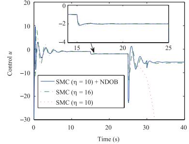
(35) In order to show the advantages of the NDOB-based SMC method proposed in this paper compared with the nominal sliding control, we will use simulations to compare the performance between them for (35). The control parameters of the two control methods are listed in Table Ⅰ. Consider the initial states of (35) as . Mismatched/matched uncertainties and disturbances ${d_1} = 1.5, {d_2} = 0.5, {d_3} = 1$ are imposed on the system at 25, 30, 15 sec respectively. The simulation results are shown in Figs. 2-4.
表 Ⅰ Control Parameters for the Numerical Example in Case 1Table Ⅰ Control Parameters for the Numerical Example in Case 1Controllers Parameters SMC1 k = 8, η= 16 SMC2 k = 8, η= 10 NDOB-SMC k = 8, η = 10, l = diag{6, 6, 6} 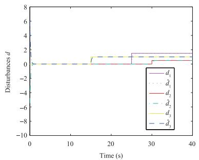 图 4 Reference/estimation uncertainties and disturbances.Fig. 4 Reference/estimation uncertainties and disturbances.
The reference/estimation uncertainties and disturbances of the system are shown in Fig. 4. It can be seen from Fig. 4 that the proposed control gives a better estimation of the disturbance and a better performance.
4.2 Application to PMSM Speed Control System
In $d-q$ coordinates the permanent magnet synchronous motor (PMSM) dynamic equation can be written as
$ \begin{equation} \dot \omega = - a\omega + b{i_q} - d \end{equation} $
(36) where $a = B/J$ , $b = 3p{\psi _f}/{(2J)}$ , $d = T_L/J$ . $\omega$ is the rotor angular velocity, $p$ is the number of pole pairs, ${\psi _f}$ is the flux linkage, ${T_L}$ is the load torque, $B$ is the viscous friction coefficient, $J$ is the moment of inertia.
The state variable of speed error is defined as and its derivative as follows:
$ \begin{equation} {\dot x_1} = {x_2} = {\dot \omega _{\rm ref}} - \dot \omega = {\dot \omega _{\rm ref}} + a\omega - b{i_q} + d \end{equation} $
(37) where ${\omega _{\rm ref}}$ is the reference speed signal.
The speed error derivative dynamic equation of the motor can be expressed as follows, with the parameters variations taken into account:
$ \begin{eqnarray} {{\dot x}_1} & = & {{\dot \omega }_{\rm ref}} + a\omega + \Delta a\omega - b{i_q} - \Delta b{i_q} + d + \Delta d\nonumber\\ & = & {x_2} + \Delta a\omega - \Delta b{i_q} + \Delta d\nonumber\\ & = & {x_2} + {d_1} \end{eqnarray} $
(38) where $\Delta a$ , $\Delta b$ , and $\Delta d$ are parameter variations of $a$ , $b$ , $d$ , and is considered as mismatched uncertainties.
The second-order model of speed error derivative dynamic equation of PMSM system is described by
$ \begin{equation} {\dot x_2} = {\ddot \omega _{\rm ref}} - \ddot \omega = {\ddot \omega _{\rm ref}} + a\dot \omega - b{\dot i_q} + \dot d. \end{equation} $
(39) ${\dot x_2}$ can be expressed as follows, with the parameters variations taken into account:
$ \begin{eqnarray} {{\dot x}_2} & = & {{\ddot \omega }_{\rm ref}} + a\dot \omega + \Delta a\dot \omega - b{{\dot i}_q} - \Delta b{{\dot i}_q} + \dot d + \Delta \dot d\nonumber\\ & = & - a{x_2} - b{{\dot i}_q} + {d_2}\nonumber\\ & = & - a{x_2} - bu + {d_2} \end{eqnarray} $
(40) where $u = {\dot i_q}$ , .
The second-order model of the PMSM speed regulation system can be represented in the following state-space form:
$ \begin{equation} \left\{ \begin{array}{l} {{\dot x}_1} = {x_2} + {d_1}\\ {{\dot x}_2} = - a{x_2} - bu + {d_2} \end{array} \right.. \end{equation} $
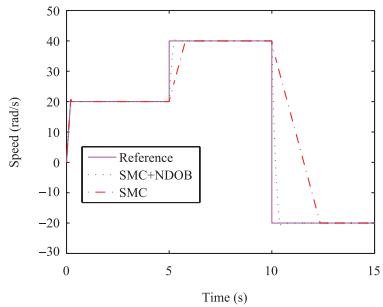
(41) To demonstrate the efficiency of the proposed method, simulation studies are carried out in this section. The parameters of the PMSM are given as follows: ${R_s} = 1.62 \Omega $ , ${L_d} = {L_q}$ = 0.005 H, B = 7.403 $\times {10^{ - 5}}$ N $\cdot$ m $\cdot$ s/rad, $J = 1.74 \times {10^{ - 4}}$ kg $\cdot$ m $^2$ , ${\psi _f}$ = 1.608 wb, $p =2$ . The control parameters of the two control methods are listed in Table Ⅱ. The simulation results are shown in Figs. 5-8.
表 Ⅱ Control Parameters for the Numerical Example in Case 2Table Ⅱ Control Parameters for the Numerical Example in Case 2Controllers Parameters SMC1 k = 8000, η= 950 NDOB-SMC k = 8000, η = 950, l = diag{6, 6}  图 8 Speed curve under variable parameter.Fig. 8 Speed curve under variable parameter.
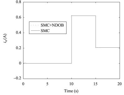
Fig. 5 depicts the variable curve, reference speed changes from 20 rad/s to 40 rad/s at 5 s, and 40 rad/s to -20 rad/s at 10 s. It can be observed that the proposed method exhibits a faster speed and smooth transition than the nominal SMC method.
The unknown load torque ${T_L}$ = 3 N $\cdot$ m is supposed to add to the PMSM at 10 s, and be removed from the system at 15 s. Response curves of the rotor speed, q-axis currents are shown in Figs. 6 and 7. It can be seen that the proposed control method obtains fine tracking performance in the presence of unknown external load torque variations.
The response curves of the PMSM under the proposed method in the presence of mechanical parameter variations are shown in Fig. 8. The moment of inertia is supposed to have variations in its nominal operation values, 2 J at 10 s, and 1.5 J at 15 s, respectively. It can be observed from Fig. 8 that the proposed method is insensitive to mismatched uncertainty, and has fine robustness performance, while the nominal SMC method is sensitive to mismatched uncertainty.
5. Conclusion
In this paper, the mismatched/matched uncertainties and disturbances rejection control problem have been studied for the second-, third-, and higher-order systems. A novel NDOB-based SMC approach has been proposed. The controller not only make the states of closed-loop system obtain better tracking performance, but also enhance the disturbance attenuation and system robustness. The proposed method has exhibited nominal performance recovery and chattering reduction as compared with the nominal SMC. Simulation results reveal the effectiveness of the proposed method.
-
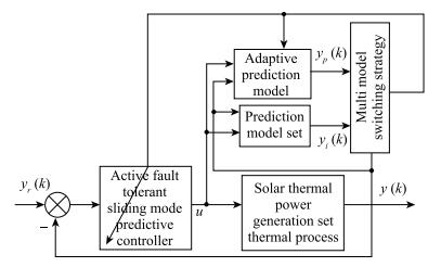
Fig. 2 The structure of a multi-model active fault tolerant controller of solar thermal power generation.
Table Ⅰ Clustering Results
C 2 3 4 5 6 7 8 9 DB 1.3893 1.0168 0.6306 0.7065 0.1746 0.9135 0.4936 0.6304  下载: 导出CSV
-
[1] E. F. Camacho, F. R. Rubio, M. Berenguel, L. Valenzuela, "A survey on control schemes for distributed solar collector fields. Part Ⅰ: modeling and basic control approaches, " Solar Energy, vol. 81, no. 10, pp. 1240-1251, Oct. 2007. http://www.researchgate.net/publication/222647936_A_survey_on_control_schemes_for_distributed_solar_collector_fields._Part_II_Advanced_control_approaches [2] M. Pasamontes, J. D. Álvarez, J. L. Guzmán, J. M. Lemos, M. Berenguel, "A switching control strategy applied to a solar collector field, " Control Eng. Pract. , vol. 19, no. 2, pp. 135-145, Feb. 2011. https://www.researchgate.net/publication/229350105_A_switching_control_strategy_applied_to_a_solar_collector_field [3] G. A. Andrade, D. J. Pagano, J. D. Álvarez, M. Berenguel, "A practical NMPC with robustness of stability applied to distributed solar power plants, " Solar Energy, vol. 92, pp. 106-122, Jun. 2013. https://www.researchgate.net/publication/236027498_A_practical_NMPC_with_robustness_of_stability_applied_to_distributed_solar_power_plants [4] P. Gil, J. Henriques, A. Cardoso, P. Carvalho, A. Dourado, "Affine neural network-based predictive control applied to a distributed solar collector field, " IEEE Trans. Control Syst. Technol. , vol. 22, no. 2, pp. 585-596, Mar. 2014. https://www.researchgate.net/publication/259190830_Affine_Neural_Network-Based_Predictive_Control_Applied_to_a_Distributed_Solar_Collector_Field [5] M. Gálvez-Carrillo, R. De Keyser, C. Ionescu, "Nonlinear predictive control with dead-time compensator: application to a solar power plant, " Solar Energy, vol. 83, no. 5, pp. 743-745, May 2009. https://www.researchgate.net/publication/229341885_Nonlinear_predictive_control_with_dead-time_compensator_Application_to_a_solar_power_plant [6] B. C. Torrico, L. Roca, J. E. Normey-Rico, J. L. Guzman, L. Yebra, "Robust nonlinear predictive control applied to a solar collector field in a solar desalination plant, " IEEE Trans. Control Syst. Technol. , vol. 18, no. 6, pp. 1430-1439, Nov. 2010. https://www.researchgate.net/publication/224106832_Robust_Nonlinear_Predictive_Control_Applied_to_a_Solar_Collector_Field_in_a_Solar_Desalination_Plant [7] A. J. Gallego, E. F. Camacho, "Adaptative state-space model predictive control of a parabolic-trough field, " Control Eng. Pract. , vol. 20, no. 9, pp. 904-911, Sep. 2012. https://www.researchgate.net/publication/257427102_Adaptative_state-space_model_predictive_control_of_a_parabolic-trough_field [8] A. Zakharov, E. Zattoni, M. Yu, S. L. Jämsä-Jounela, "A performance optimization algorithm for controller reconfiguration in fault tolerant distributed model predictive control, " J. Process Control, vol. 34, pp. 56-69, Oct. 2015. https://www.researchgate.net/publication/304285479_A_performance_optimization_algorithm_for_controller_reconfiguration_in_fault_tolerant_distributed_model_predictive_control [9] X. Du, Y. Q. Guo, X. L. Chen, "MPC based active fault tolerant control of a commercial turbofan engine, " J. Propuls. Technol. , vol. 36, no. 8, pp. 1242-1247, Aug. 2015. https://www.researchgate.net/publication/283020143_MPC_based_active_fault_tolerant_control_of_a_commercial_turbofan_engine [10] S. V. Naghavi, A. A. Safavi, M. Kazerooni, "Decentralized fault tolerant model predictive control of discrete-time interconnected nonlinear systems, " J. Franklin Inst. , vol. 351, no. 3, pp. 1644-1656, Mar. 2014. https://www.researchgate.net/publication/259504884_Decentralized_Fault_Tolerant_Model_Predictive_Control_of_Discrete-Time_Interconnected_Nonlinear_Systems [11] R. Carmona, Analysis, Modeling and Control of a Distributed Solar Collector Field with a One-Axis Tracking System; . Spanish: University of Seville, 1985, pp. 18-34. [12] K. L. Zhou, S. L. Yang, S. Ding, H. Luo, "On cluster validation, " Syst. Eng. Theory Pract. , vol. 34, no. 9, pp. 2417-2431, Sep. 2014. http://en.cnki.com.cn/Article_en/CJFDTOTAL-XTLL201409027.htm [13] X. C. Wang, F. Shi, L. Yu, Li Y, 43 Case Analysis of MATLAB Neural Network. Beijing: Beihang University Press, 2013. [14] D. L. Davies, D. W. Bouldin, "A cluster separation measure, " IEEE Trans. Pattern Anal. Mach. Intell. , vol. PAMI-1, no. 2, pp. 224-227, Apr. 1979. [15] P. Lu, P. Van Eykeren, E. Van Kampen, Q. P. Chu, "Selective-reinitialization multiple-model adaptive estimation for fault detection and diagnosis, " J. Guid. Control, Dyn. , vol. 38, no. 8, pp. 1409-1424, 2015. https://www.researchgate.net/publication/275044066_Selective-Reinitialization_Multiple-Model_Adaptive_Estimation_for_Fault_Detection_and_Diagnosis [16] A. Mohammadi, K. N. Plataniotis, "Improper complex-valued multiple-model adaptive estimation, " IEEE Trans. Signal Process. , vol. 63, no. 6, pp. 1528-1524, Mar. 2015. https://www.researchgate.net/publication/271194732_Improper_Complex-Valued_Multiple-Model_Adaptive_Estimation [17] H. Y. Gao, Y. L. Cai, "Sliding mode predictive control for hypersonic vehicle, " J. Xi'an Jiaotong Univ. , vol. 48, no. 1, pp. 67-72, Jan. 2014. http://en.cnki.com.cn/Article_en/CJFDTotal-XAJT201401012.htm [18] Z. G. Miao, S. S. Xie, L. Wang, J. B. Peng, X. S. Zhai, "Multi-model predictive sliding mode control for aero-engine, " J. Propuls. Technol. , vol. 33, no. 3, pp. 472-477, Jun. 2012. http://en.cnki.com.cn/article_en/cjfdtotal-tjjs201203021.htm [19] H. Yang, K. P. Zhang, X. Wang, "Multi-model switching predictive control with active fault tolerance for high-speed train, " Control Theory Appl. , vol. 29, no. 9, pp. 1211-1214, Sep. 2012. http://en.cnki.com.cn/Article_en/CJFDTotal-KZLY201209018.htm -

 下载:
下载:


计量
- 文章访问数: 1848
- HTML全文浏览量: 219
- PDF下载量: 757
- 被引次数: 0
