

Application of Multi-model Active Fault-tolerant Sliding Mode Predictive Control in Solar Thermal Power Generation System
-
Abstract: To address the stability of solar thermal power generation system which is characterized by the presence of random and strong disturbance, a multi-model active fault-tolerant controller is designed in this paper. Actually measured data is used to make fuzzy clustering, then multi-model of the collector subsystem is established through recursive least square method. A switching strategy based on the minimum cumulative error is applied to select the optimal control model online. In order to reduce the error caused by missing data, fault and strong disturbance in the process of building the multi-model, the adaptive prediction model of solar collector system is established. Active fault tolerant sliding mode predictive controller is designed to improve the tracking accuracy and robustness of the output. Finally, the validity and advantage of the proposed algorithm are verified.
-
Key words:
- Active fault-tolerant control /
- adaptive switching /
- fuzzy clustering /
- multi-model /
- solar thermal power generation
-
Solar thermal power generation system is affected by natural factors such as solar radiation, and also the system has strong interference. These uncertain factors directly affect the quality of solar thermal power generation. Regulating the tracking error of output oil temperature of collector is an important control objective, therefore it has practical significance to study the active fault tolerant predictive control of solar collector system in the state of fault or disturbance.
The solar collector system uses the solar radiation to heat the heat conduction oil, regulates the flow of heat conduction oil, and controls the outlet temperature of the heat conduction oil in a certain range so as to ensure the stability of the power generation. The control objective of the collection system is that the amount of the actual output is as close as possible to the amount of the desired target output. In recent years, many kinds of intelligent control algorithms are applied to the control of solar thermal power generation system [1]-[3]. Reference [4]-[7] all applied the model predictive control algorithm, where the control target was to minimize the tracking error.
Error of the outlet temperature and the single model are used to predict the model. Multi-model adaptive switching active fault tolerant control is about selecting the model with least cumulative error to determine which model of multi-models is the best match for the dynamic behavior of the system online, and continuously optimize the model parameters. The adaptive model which can be reassigned is used to compensate for the missing data in the process of modeling and to reduce the tracking error with strong disturbance or fault conditions. The algorithm has been successfully applied to other areas [8]-[10], the control effect is good. Based on the above analysis, the main research contents of this paper include:
1) Establish multi-model set. Collect data sets for several consecutive days to make the fuzzy C-means (FCM) clustering.
2) Design active fault tolerant sliding mode predictive controller. Determine the adaptive switching strategy. The inlet temperature and solar radiation are considered as disturbance, and flow of heat conduction oil is considered as controlled variable. Based on the multi-model, the adaptive model of the solar collector system is established to adapt the object and the disturbance characteristics. A model switching strategy based on the minimum cumulative error is used to select the optimal control model online.
3) The method is applied to the actual linear Fresnel power generation system, and the method is compared with [3]. The method in this paper is better than the method [3], the control precision is higher, and the time delay is shorter.
1. Dynamic Model of Solar Thermal Power Generation System
1.1 The Mathematical Model of Micro-sources
1.1.1 Microturbine Cost
R Carmona, a Spanish scholar, initially used the mathematical model [1] to describe the temperature of heat conduction oil of the solar collector [11], and then the model was used to analyze the thermal system [4]-[6].
$ \begin{align} & {\rho _{\rm{f}}}{C_{\rm{f}}}{A_{\rm{f}}}\frac{{{d}{T_n}(t)}}{{{{d}}t}} = {\eta _{\rm{0}}}{G_1}I(t) - {\rho _{\rm{f}}}{C_{\rm{f}}}v(t)\frac{{{T_n}(t) - {T_{n - 1}}(t)}}{{\Delta x}}, \nonumber\\ & \;\;\;\;\;\;\; n = 1, \ldots, N \end{align} $
(1) where $t$ is time, s; $\Delta x$ is length of the collector tube section; ${\rho _{\rm{f}}}$ is refrigerant density, kg/m $^3$ ; ${C_{\rm{f}}}$ is specific heat capacity, ; ${A_{\rm{f}}}$ is cross section area of pipe; $v(t)$ is conduction heat oil flow, ${\rm m^3}$ /s; $I(t)$ is solar intensity, W/ ${\rm m^2}$ ; ${\rm \eta _0}$ is mirror optical efficiency; ${G_1}$ is the optical aperture of reflector, m; $Tn$ is conduction heat oil temperature of oil pipeline outlet, ℃; $Tn - 1$ is conduction heat oil temperature of oil pipeline outlet, ℃.
Take $\Delta x$ = $L$ , then (1) can be
$ \begin{align} & {\rho _{\rm{f}}}{C_{\rm{f}}}{A_{\rm{f}}}\frac{{{\rm{d}}{T_n}(t)}}{{{\rm{d}}t}} = {\eta _{\rm{0}}}{G_1}I(t) - {\rho _{\rm{f}}}{C_{\rm{f}}}v(t)\frac{{{T_n}(t) - {T_0}(t)}}{L}, \notag\\ & \;\;\;\;\;\;\quad n = 1, \ldots, N \end{align} $
(2) where $L$ is the total length of pipeline of the collection system; $T{}_0(t)$ is the entrance conduction heat oil temperature of collector.
2. Clustering Modeling of Solar Thermal Power Generation Set
2.1 Fuzzy Clustering of Data Set
The data acquisition in the linear Fresnel thermal power generation system is used to make FCM clustering analysis. In this clustering algorithm, the membership degree is used to determine the degree of each element and the measured data is classified by the method of subtraction clustering [12], [13].
Step 1: Determine the number of categories $C$ , fuzzy weight index m and the initial clustering center $v$ ;
Step 2: The fuzzy membership degree ${u_{ij}}$ is calculated according to
$ \begin{align} {u_{ij}} = \begin{cases} {\left[{\sum\limits_{k = 1}^C {\frac{{{{\left\| {{x_i}-{\upsilon _j}} \right\|}^{\frac{2}{{m-1}}}}}}{{{{\left\| {{x_i}-{\upsilon _k}} \right\|}^{\frac{2}{{m - 1}}}}}}} } \right]^{ - 1}}, & \left\| {{x_i} - {\upsilon _k}} \right\| \ne 0\\ 1, & \left\| {{x_i} - {\upsilon _k}} \right\| = 0, ~~{k} = j\\ 0, & \left\| {{x_i} - {\upsilon _k}} \right\| = 0, ~~{k} \ne j. \end{cases} \end{align} $
(3) ${u_{ij}}$ is the fuzzy membership degree of category $J$ of individual. ${\upsilon _j}$ is cluster center of category $J$ .
Step 3: Use (4) to calculate the center of each category.
$ \begin{align} {\upsilon _j} = \frac{{\sum\limits_{i = 1}^n {u_{ij}^m{x_i}} }}{{\sum\limits_{i = 1}^n {u_{ij}^m} }}. \end{align} $
(4) Step 4: The target value is calculated according to (5) to determine whether the values meet the target value or not. If the values meet the target value, the clustering is end. Otherwise, return Step 2.
$ \begin{align} J = \sum\limits_{i = 1}^n {\sum\limits_{j = 1}^C {{{({u_{ij}})}^m}\left\| {{x_i} - {\upsilon _j}} \right\|} }. \end{align} $
(5) In this paper, DB is used as an evaluation index of the classification [14]. The smaller the index value is, the better the clustering effect is. In this paper, for 3500 sets of actual power generation data $M$ from the solar thermal power generation system of Gansu Lanzhou Dacheng company, which is put into use in Lanzhou New District, $M({m_1}$ , ${m_2}$ , ${m_3}$ , ${m_4}$ ) is classified, among them, ${m_1}$ is the outlet temperature, ${m_2}$ is the heat transfer oil outlet temperature, ${m_3}$ is flow, and the solar radiation is ${m_4}$ . Fuzzy clustering is used to analyze such data. When $C$ = 6, DB is the smallest, and Table Ⅰ lists the clustering results.
表 Ⅰ Clustering ResultsTable Ⅰ Clustering ResultsC 2 3 4 5 6 7 8 9 DB 1.3893 1.0168 0.6306 0.7065 0.1746 0.9135 0.4936 0.6304 The clustering centers of the 6 types are respectively:
$ \begin{align*} & {\upsilon _1} = (\begin{array}{*{20}{c}} {236.6} & {196.0} & {10.15} & {780.5} \end{array})\\ & {\upsilon _2} = (\begin{array}{*{20}{c}} {244.4} & {203.0} & {10.03} & {890.9} \end{array})\\ & {\upsilon _3} = (\begin{array}{*{20}{c}} {250.1} & {210.0} & {10.20} & {916.6} \end{array})\\ & {\upsilon _4} = (\begin{array}{*{20}{c}} {253.6} & {213.4} & {10.32} & {933.0} \end{array})\\ & {\upsilon _5} = (\begin{array}{*{20}{c}} {259.7} & {219.6} & {10.18} & {935.5} \end{array})\\ & {\upsilon _6} = (\begin{array}{*{20}{c}} {273.6} & {232.9} & {10.04} & {953.2} \end{array}). \end{align*} $
2.2 Least-squares Modeling
The above classification data results considered the inlet oil temperature, solar radiation and flow rate of conduction heat oil as input, and outlet temperature as output. In order to overcome the shortcomings of the least squares due to its poor correction ability, forgetting factor recursive least square method is adopted [9], [15], [16]. The controlled auto regressive (CAR) model expressed by formula (6) is used to identify the parameters.
$ \begin{align} y(k) = {{\bf{\varphi }}^T}(k)\hat\theta (k). \end{align} $
(6) where,
$ \begin{align*} & y(k + 1) = [{y_1}(k + 1), {y_2}(k + 1), {y_3}(k + 1), \\ & \;\;\quad {y_4}(k + 1), {y_5}(k + 1), {y_6}(k + 1){]^{{T}}} \\[3mm] & \hat\theta = \left[{\begin{array}{*{20}{c}} {{a_{11}}} & {{a_{12}}} & {{a_{13}}} & {{a_{14}}}\\ {{a_{21}}} & {{a_{22}}} & {{a_{23}}} & {{a_{24}}}\\ {{a_{31}}} & {{a_{32}}} & {{a_{33}}} & {{a_{34}}}\\ {{a_{41}}} & {{a_{42}}} & {{a_{43}}} & {{a_{44}}}\\ {{a_{51}}} & {{a_{52}}} & {{a_{53}}} & {{a_{54}}}\\ {{a_{61}}} & {{a_{62}}} & {{a_{63}}} & {{a_{64}}} \end{array}} \right]\nonumber \\[3mm] & {{ {\varphi }}^T}(k + 1) = \left[{\begin{array}{*{20}{c}} {-{y_1}(k)} & {{u_1}(k)} & {{T_{\rm out}}_1(k)} & {{I_1}(k)}\\ {-{y_2}(k)} & {{u_2}(k)} & {{T_{\rm out2}}(k)} & {{I_2}(k)}\\ {-{y_3}(k)} & {{u_3}(k)} & {{T_{\rm out3}}(k)} & {{I_3}(k)}\\ { - {y_4}(k)} & {{u_4}(k)} & {{T_{\rm out4}}(k)} & {{I_4}(k)}\\ { - {y_5}(k)} & {{u_5}(k)} & {{T_{\rm out5}}(k)} & {{I_5}(k)}\\ { - {y_6}(k)} & {{u_6}(k)} & {{T_{\rm out6}}(k)} & {{I_6}(k)} \end{array}} \right].\nonumber \end{align*} $
Initial value $\theta (0) = 0$ is the positive real vector with zero or small value. The mathematical model of the solar collector system can be obtained, as shown in the model (7).
$\begin{align} \begin{cases} {y_1}(k + 1) = 0.9217{y_1}(k) + 0.3011{u_1}(k)\\ \;\;\quad +~ 0.0701{T_{\rm in}}_1(k) + 0.0015{I_1}(k)\\[2mm] {y_2}(k + 1) = 0.9501{y_2}(k) + 0.2126{u_2}(k)\\ \;\;\quad +~ 0.0631{T_{\rm in2}}(k) + 0.0041{I_2}(k)\\[2mm] {y_3}(k + 1) = 0.9438{y_3}(k) + 0.6421{u_3}(k)\\ \;\;\quad +~ 0.0763{T_{\rm in}}_3(k) + 0.0039{I_3}(k) \\[2mm] {y_4}(k + 1) = 0.9573{y_4}(k) + 0.434{u_4}(k)\\ \;\;\quad +~ 0.0614{T_{\rm in4}}(k) + 0.0032{I_4}(k) \\[2mm] {y_5}(k + 1) = 0.9680{y_5}(k) + 0.3171{u_5}(k)\\ \;\;\quad +~ 0.0549{T_{\rm in5}}(k) + 0.0036{I_5}(k) \\[2mm] {y_6}(k + 1) = 0.9702{y_6}(k) + 0.4021{u_6}(k)\\ \;\;\quad +~ 0.0593{T_{\rm in6}}(k) + 0.0031{I_6}(k) \end{cases} \end{align} $
(7) where ${y_i}(k)$ is output oil temperature, ${u_i}(k)$ is the flow rate of conduction heat oil, ${T_{\rm in}}_{ i}(k)$ is input oil temperature, and ${I_i}(k)$ is solar radiation.
According to the results of the optimal clustering center, the outlet temperature is considered as the center to analyze the error of classification. Fig. 1 shows the effect of deviation of each class of data from the center point of the cluster. In different temperature and cross sectional output data, outlet temperature is also affected by the inlet temperature and solar radiation. Therefore, the system can be considered as a multi disturbance system.
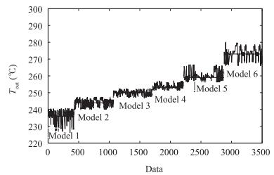 图 1 Error of multi-model and clustering center.Fig. 1 Error of multi-model and clustering center.
3. Multi-model Active Fault Tolerant Sliding Mode Predictive Controller
Predictive control includes prediction model, rolling optimization and feedback correction. Under the condition of system fault or disturbance, the multi-model adaptive switching active fault tolerant control can update the control law based on the optimal predictive model online, which results in stable operation of the closed-loop system. In the process of rolling optimization, update control law online, and through the feedback of correction, the error is corrected online. Fig. 2 is the structure of a multi-model active fault tolerant controller of solar thermal power generation. ${y_r}(k)$ is the desired output, $y(k)$ is the actual output of model, ${y_i}(k)$ is the most optimal sub model, and ${y_p}(k)$ is the adaptive model.
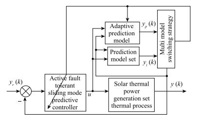 图 2 The structure of a multi-model active fault tolerant controller of solar thermal power generation.Fig. 2 The structure of a multi-model active fault tolerant controller of solar thermal power generation.
In [17]-[19], a single model sliding mode predictive control is designed for the high speed aircraft. In [18], a multi-model sliding mode predictive control is designed for the disturbance signal. Active fault tolerant predictive controller is designed for high-speed train based on [19]. In the literature, the designed controller according to different system has achieved good control effect. By referring to the above documents, this article designed the active fault tolerant control in solar thermal applications. Consider the following uncertain discrete linear systems
$ \begin{align} y(k + 1) - {{{A}}}y(k) = {{{B}}}u(k) + \xi (k) \end{align} $
(8) where $y(k)$ is the output, $u(k)$ $\in \mathbb{R}$ is the control input, $A$ and $B$ are matrixes with appropriate dimension, and is the total interference.
3.1 Sliding Mode Surface Design
Define the switching function: set the reference command signal ${y_r}(k)$ , define the tracking error (9).
$ \begin{align} e(k) = y(k) - {y_r}(k). \end{align} $
(9) Define the linear switching function:
$ \begin{align} s(k) = {\sigma ^{T}}e(k) \end{align} $
(10) where ${\sigma ^{T}} = [{\sigma _1}, \ldots, {\sigma _n}]$ . After the solar collector model expression (2) is discretized, the configuration of poles of the expected oil outlet temperature is set inside the unit circle, and then ${\sigma _i}$ is obtained through the calculation. In order to guarantee the stability and dynamic performance of the ideal sliding mode, construct the following sliding mode prediction model.
$ \begin{align} s(k + 1) = {\sigma ^{T}}e(k + 1). \end{align} $
(11) The predicted sliding mode surface is ${S_m} = \{ e(k)|{s(e(k))}$ $=$ $0\}$ . The p step ahead predictor is as follow.
$ \begin{align} s(k + p) = & \ {\sigma ^{T}}{A^p}y(k)\nonumber\\ & + \sum\limits_{i = 1}^p {{\sigma ^{T}}{A^{p - i}}[} Bu(k + p-i)\nonumber\\ & + \xi (k + p-i)] - {\sigma ^{T}}{y_r}(k + p). \end{align} $
(12) Use the difference value between actual switching function output value $s(k)$ and $p$ step ahead prediction at the moment of $k - p$ to make the feedback correction of output value ${s_p}(k + p)$ of sliding mode prediction model. Thus, the output of the closed-loop sliding mode prediction model can be expressed as:
$ \begin{align} {{\tilde s}_p}(k + p) = s(k + p) + {\zeta _p}[s(k)-{s_p}(k | {k- p})] \end{align} $
(13) where ${\zeta _p} \in \mathbb{R}$ is the weighted feedback correction factor. Let ${\zeta _1}$ $=$ $1$ , $0 < {\zeta _p} < 1$ $(p \ge 1)$ . Decrease of ${\zeta _p}$ can reduce the role of feedback correction.
3.2 Sliding Mode Reference Trajectory
Take the commonly reaching rate as the reference trajectory.
$ \begin{align} \begin{cases} {s_r}(k + p) = \mu {s_r}(k + p - 1) + \eta {\rm sgn} ({s_r}(k + p - 1))\\ {{s_r}(k) = s(k)} \end{cases} \end{align} $
(14) where $0 < \mu < 1, $ $\eta >0$ . The greater the $\mu $ , the smaller the switching power. Control objective is that the error state reaches the sliding mode surface that is to say $s(e(k)) = 0$ .
3.3 Control Law Design
Define the performance index
$ \begin{align} J= \sum\limits_{i = 1}^N {{{({s_r}(k + i) - \tilde s(k + i))}^2}} + \sum\limits_{j = 0}^{M - 1} {{\lambda _j}{u^2}(k + j)} \end{align} $
(15) where $N$ and $M$ are positive integers, which respectively represent the predicted time domain and control time domain, $M$ needs to meet $N< 0 < M, $ $u(k + j) = u(k + M - 1)$ , $M $ $\le$ $j$ $<$ $ N$ , and ${\lambda _j}$ is weight coefficient.
If the output vector is expressed as:
$ \begin{align} & S = {[s(k + 1), \ldots, s(k + N)]^{T}}\;\;\nonumber \\ & {S_r} = {[{s_r}(k + 1), \ldots, {s_r}(k + N)]^{T}}\nonumber \\ & \tilde S = {[{\tilde s_{}}(k + 1), \ldots, \tilde s(k + N)]^{T}}\;\;\;\nonumber \\ & \bar S = {[s(k)-{s_p}(k\left| {k-1} \right.), \ldots, s(k)-{s_p}(k\left| {k - N} \right.)]^{T}}\notag\\ & \ \ = {[\bar S(1), \ldots, \bar S(N)]^{T}}\notag\\ & U = {[u(k), \ldots, u(k + M-1)]^{T}}\notag\\ & F = {[{\sigma ^{T}}A, \ldots, {\sigma ^{T}}{A^N}]^{T}}\; \nonumber \\ & \Xi = {\rm diag}\{ {\zeta _1}, \ldots, {\zeta _N}\} \notag\\ & \Lambda = {\rm diag}\{ {\lambda _1}, \ldots, {\lambda _M}\}\notag\\ & {{\tilde Y}_r} = {[{{\tilde y}_r}(k), \ldots, {{\tilde y}_r}(k + N -1)]^{T}} \nonumber \end{align} $
$ \begin{array}{l} G = \left[{\begin{array}{*{20}{c}} {{\sigma ^T}B} & 0 & \cdots & 0\\ {{\sigma ^T}AB} & {{\sigma ^T}B} & \cdots & 0\\ \vdots & \vdots & \cdots & {{\sigma ^T}B}\\ \vdots & \vdots & \ddots & \vdots \\ {{\sigma ^T}{A^{N-2}}B} & {{\sigma ^T}{A^{N-3}}B} & \cdots & {\sum\limits_{i = 0}^{N-M - 1} {{\sigma ^T}{A^i}B} }\\ {{\sigma ^T}{A^{N - 1}}B} & {{\sigma ^T}{A^{N - 2}}B} & \cdots & {\sum\limits_{i = 0}^{N - M} {{\sigma ^T}{A^i}B} } \end{array}} \right]\\ P = \left[{\begin{array}{*{20}{c}} {{\sigma ^T}} & 0 & \cdots & 0\\ {{\sigma ^T}A} & {{\sigma ^T}} & \cdots & 0\\ \vdots & \vdots & \ddots & \vdots \\ {{\sigma ^T}{A^{N-1}}} & {{\sigma ^T}{A^{N-2}}} & \cdots & {{\sigma ^T}} \end{array}} \right] \end{array} $
then (12) and (13) can be represented as a vector form, which can be expressed by (16) and (17).
$ \begin{array}{l} & S = Fe(k) + GU + P{\tilde Y_r}\;\; \end{array} $
(16) $ \begin{align} & \tilde S = S + \Xi \bar S.\;\;\;\; \end{align} $
(17) So, the performance index expressed by(15) can be written as a vector form expressed by (18).
$ \begin{align} J = {(H - GU)^{T}}(H - GU) + \Lambda {U^{T}}U \end{align} $
(18) where ${L_0}=$ $[1, $ $\ldots, 1]^{T}, $ ${L_1} = {[{\gamma ^1}, \ldots, {\gamma ^N}]^{T}}, $ $ 0 $ $< \gamma$ $<$ $1, $ .
Let $\frac{{\partial J(U)}}{{\partial U}} = 0$ , solve the corresponding equations, and the optimal flow rate of $U$ in the collection process is calculated:
$ \begin{align} U = {({G^{T}}G + \Lambda)^{ - 1}}{G^{T}}H. \end{align} $
(19) 3.4 Multi-model Switching Strategy
The switching strategy is to select the optimal control model online [18] for the state of system under the condition of unknown fault or disturbance, and the active fault tolerant predictive control is carried out through the rolling optimization and feedback correction.
At the $k$ th moment, ${e_i}(k) = y(k) - {\hat y_i}(k)$ is the output error between actual output and $i$ $(1 \le i \le P* + 2)$ model. The definition of switching index is shown in (20).
$ \begin{align} {J_i}(k) = \alpha e_i^2(k) + \beta \sum\limits_{j = 1}^L {{\theta ^j}e_i^2(k - j)} \end{align} $
(20) where $\alpha $ is error coefficient at present, $\beta $ error coefficient for historical moment, $\alpha > 0, $ $\beta > 0, $ $\alpha + \beta = 1$ , $L$ is the number of the concerned historical sampled data, and $\theta = 1$ .
3.5 Adaptive Fault-tolerant Control
3.5.1 Active Fault-tolerant Algorithm
Under the condition of system failure or disturbance, the active fault tolerant control can update the control law according to the optimal control model online selection, which can stabilize the closed loop system [19]. Active fault tolerant control is realized by the adaptive model switching.
3.5.2 Adaptive Model Switching
The adaptive model can be used to obtain a faster convergence rate according to the different conditions. According to the model switching strategy, if the initial parameters of the model are the optimal model parameters of the multi-model set, the optimal model can be selected from the current optimal model set and the parameters can be updated with (21). Otherwise, the initial value of the model is reassigned to the minimum cumulative error model parameters, and then the model parameters are updated online through (21). According to the model switching strategy, the obtained optimal model is the adaptive model, which can guarantee the stability of the system and the accuracy of tracking. Parameters are updated as follows [9], [19].
$ \begin{align} \begin{cases} \hat \theta (k) = \hat \theta (k - 1) + K(k)[y(k)-{\varphi ^T}(k)\hat \theta (k- 1)]\\[1mm] K\left( k \right) = \dfrac{{P\left( {k - 1} \right)\varphi \left( k \right)}}{{\lambda + {\varphi ^T}\left( k \right)P\left( {k - 1} \right)\varphi \left( k \right)}}\\[3mm] P(k) = \dfrac{1}{\lambda }\left[I-K(k){\varphi ^T}(k)\right]P(k - 1) \end{cases} \end{align} $
(21) where $\theta (k)$ are the parameters to be identified, $K(k)$ is gain matrix, $\varphi (k)$ is observation matrix, $P(k)$ is covariance matrix, and $\lambda $ is forgetting factor.
4. Simulation Result Analysis
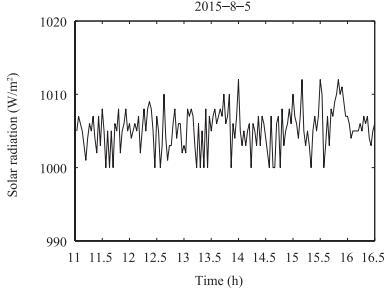
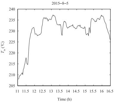
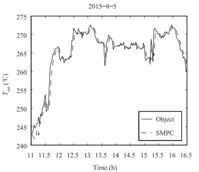
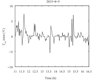
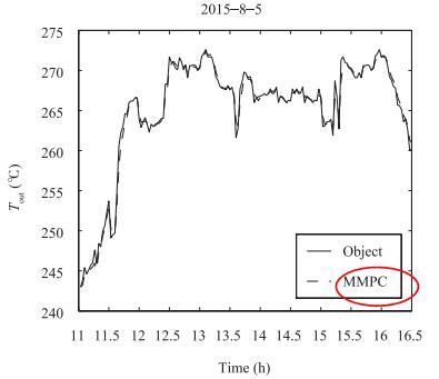
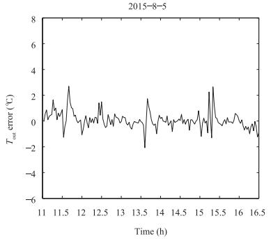
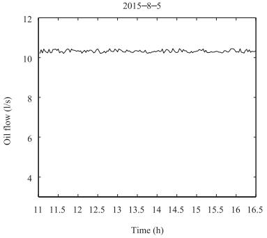
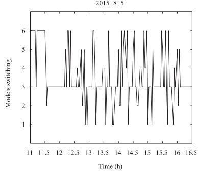
In the process of simulation analysis, system model selects (2). Parameters of the linear Fresnel power generation demonstration project in the west of China are selected and the outlet oil temperature of conducting oil on August 5, 2015 is taken as the target curve. Controlled variable is the flow of heat conduction oil. Inlet oil temperature and solar radiation are disturbances which can be measured. The flow range of heat conduction oil is 3 (l/s)-12 (l/s). ${\eta _0} = 0.60, $ ${C_f}$ $=$ $2600 {\rm J/kg}{^\circ}{\rm C}, $ $T = 20$ s, $L = 220$ m, m $^2$ , $G$ $=$ $0.80$ m. Parameter values of simulation analysis are: $\alpha$ $=$ $0.3, $ $\beta = 0.7$ , $\theta $ is the positive real vector with zero or small initial value, , and forgetting factor $\lambda $ $=$ $0.95$ . Methods in [3] are compared with this paper, the two algorithms simulation results are shown in Fig. 3 to Fig. 8. Fig. 7 and Fig. 10 are the flow of heat conductive oil, and the curve of the control value respectively. Fig. 11 is switching progress between the six models.
The average variance of two kinds of simulation results is analyzed and calculated. MSE = 1.53264 in Fig. 5 and MSE = 0.43276 in Fig. 8.
It can be seen from Fig. 7 and Fig. 10 that multi-model active fault-tolerant sliding mode predictive control is better than that of [3].
5. Conclusion
In this paper, we collected the data of 3500 sets of solar thermal power generation sets, classified them, and set up the mathematical model. A fault-tolerant sliding mode predictive controller is designed, which can reduce error, improve the system's robustness and anti-interference ability. The adaptive prediction model can be used to reduce the error caused by loss of data, the disturbance and fault.
From Fig. 5 and Fig. 8, it can be seen that the method proposed in this paper has higher accuracy and shorter lag time, and has the ability to improve the robustness and convergence rate of the solar thermal power generation system.
-
Fig. 2 The structure of a multi-model active fault tolerant controller of solar thermal power generation.
Table Ⅰ Clustering Results
C 2 3 4 5 6 7 8 9 DB 1.3893 1.0168 0.6306 0.7065 0.1746 0.9135 0.4936 0.6304  下载: 导出CSV
-
[1] E. F. Camacho, F. R. Rubio, M. Berenguel, L. Valenzuela, "A survey on control schemes for distributed solar collector fields. Part Ⅰ: modeling and basic control approaches, " Solar Energy, vol. 81, no. 10, pp. 1240-1251, Oct. 2007. http://www.researchgate.net/publication/222647936_A_survey_on_control_schemes_for_distributed_solar_collector_fields._Part_II_Advanced_control_approaches [2] M. Pasamontes, J. D. Álvarez, J. L. Guzmán, J. M. Lemos, M. Berenguel, "A switching control strategy applied to a solar collector field, " Control Eng. Pract. , vol. 19, no. 2, pp. 135-145, Feb. 2011. https://www.researchgate.net/publication/229350105_A_switching_control_strategy_applied_to_a_solar_collector_field [3] G. A. Andrade, D. J. Pagano, J. D. Álvarez, M. Berenguel, "A practical NMPC with robustness of stability applied to distributed solar power plants, " Solar Energy, vol. 92, pp. 106-122, Jun. 2013. https://www.researchgate.net/publication/236027498_A_practical_NMPC_with_robustness_of_stability_applied_to_distributed_solar_power_plants [4] P. Gil, J. Henriques, A. Cardoso, P. Carvalho, A. Dourado, "Affine neural network-based predictive control applied to a distributed solar collector field, " IEEE Trans. Control Syst. Technol. , vol. 22, no. 2, pp. 585-596, Mar. 2014. https://www.researchgate.net/publication/259190830_Affine_Neural_Network-Based_Predictive_Control_Applied_to_a_Distributed_Solar_Collector_Field [5] M. Gálvez-Carrillo, R. De Keyser, C. Ionescu, "Nonlinear predictive control with dead-time compensator: application to a solar power plant, " Solar Energy, vol. 83, no. 5, pp. 743-745, May 2009. https://www.researchgate.net/publication/229341885_Nonlinear_predictive_control_with_dead-time_compensator_Application_to_a_solar_power_plant [6] B. C. Torrico, L. Roca, J. E. Normey-Rico, J. L. Guzman, L. Yebra, "Robust nonlinear predictive control applied to a solar collector field in a solar desalination plant, " IEEE Trans. Control Syst. Technol. , vol. 18, no. 6, pp. 1430-1439, Nov. 2010. https://www.researchgate.net/publication/224106832_Robust_Nonlinear_Predictive_Control_Applied_to_a_Solar_Collector_Field_in_a_Solar_Desalination_Plant [7] A. J. Gallego, E. F. Camacho, "Adaptative state-space model predictive control of a parabolic-trough field, " Control Eng. Pract. , vol. 20, no. 9, pp. 904-911, Sep. 2012. https://www.researchgate.net/publication/257427102_Adaptative_state-space_model_predictive_control_of_a_parabolic-trough_field [8] A. Zakharov, E. Zattoni, M. Yu, S. L. Jämsä-Jounela, "A performance optimization algorithm for controller reconfiguration in fault tolerant distributed model predictive control, " J. Process Control, vol. 34, pp. 56-69, Oct. 2015. https://www.researchgate.net/publication/304285479_A_performance_optimization_algorithm_for_controller_reconfiguration_in_fault_tolerant_distributed_model_predictive_control [9] X. Du, Y. Q. Guo, X. L. Chen, "MPC based active fault tolerant control of a commercial turbofan engine, " J. Propuls. Technol. , vol. 36, no. 8, pp. 1242-1247, Aug. 2015. https://www.researchgate.net/publication/283020143_MPC_based_active_fault_tolerant_control_of_a_commercial_turbofan_engine [10] S. V. Naghavi, A. A. Safavi, M. Kazerooni, "Decentralized fault tolerant model predictive control of discrete-time interconnected nonlinear systems, " J. Franklin Inst. , vol. 351, no. 3, pp. 1644-1656, Mar. 2014. https://www.researchgate.net/publication/259504884_Decentralized_Fault_Tolerant_Model_Predictive_Control_of_Discrete-Time_Interconnected_Nonlinear_Systems [11] R. Carmona, Analysis, Modeling and Control of a Distributed Solar Collector Field with a One-Axis Tracking System; . Spanish: University of Seville, 1985, pp. 18-34. [12] K. L. Zhou, S. L. Yang, S. Ding, H. Luo, "On cluster validation, " Syst. Eng. Theory Pract. , vol. 34, no. 9, pp. 2417-2431, Sep. 2014. http://en.cnki.com.cn/Article_en/CJFDTOTAL-XTLL201409027.htm [13] X. C. Wang, F. Shi, L. Yu, Li Y, 43 Case Analysis of MATLAB Neural Network. Beijing: Beihang University Press, 2013. [14] D. L. Davies, D. W. Bouldin, "A cluster separation measure, " IEEE Trans. Pattern Anal. Mach. Intell. , vol. PAMI-1, no. 2, pp. 224-227, Apr. 1979. [15] P. Lu, P. Van Eykeren, E. Van Kampen, Q. P. Chu, "Selective-reinitialization multiple-model adaptive estimation for fault detection and diagnosis, " J. Guid. Control, Dyn. , vol. 38, no. 8, pp. 1409-1424, 2015. https://www.researchgate.net/publication/275044066_Selective-Reinitialization_Multiple-Model_Adaptive_Estimation_for_Fault_Detection_and_Diagnosis [16] A. Mohammadi, K. N. Plataniotis, "Improper complex-valued multiple-model adaptive estimation, " IEEE Trans. Signal Process. , vol. 63, no. 6, pp. 1528-1524, Mar. 2015. https://www.researchgate.net/publication/271194732_Improper_Complex-Valued_Multiple-Model_Adaptive_Estimation [17] H. Y. Gao, Y. L. Cai, "Sliding mode predictive control for hypersonic vehicle, " J. Xi'an Jiaotong Univ. , vol. 48, no. 1, pp. 67-72, Jan. 2014. http://en.cnki.com.cn/Article_en/CJFDTotal-XAJT201401012.htm [18] Z. G. Miao, S. S. Xie, L. Wang, J. B. Peng, X. S. Zhai, "Multi-model predictive sliding mode control for aero-engine, " J. Propuls. Technol. , vol. 33, no. 3, pp. 472-477, Jun. 2012. http://en.cnki.com.cn/article_en/cjfdtotal-tjjs201203021.htm [19] H. Yang, K. P. Zhang, X. Wang, "Multi-model switching predictive control with active fault tolerance for high-speed train, " Control Theory Appl. , vol. 29, no. 9, pp. 1211-1214, Sep. 2012. http://en.cnki.com.cn/Article_en/CJFDTotal-KZLY201209018.htm 期刊类型引用(0)
其他类型引用(6)
-

 下载:
下载:

计量
- 文章访问数: 1850
- HTML全文浏览量: 220
- PDF下载量: 757
- 被引次数: 6
