基于改进量子差分进化的含分布式电源的配电网无功优化

Li Yuancheng; Li Zongpu; Yang Liqun; Wang Bei

doi:10.16383/j.aas.2017.e150304

基于改进量子差分进化的含分布式电源的配电网无功优化

doi: 10.16383/j.aas.2017.e150304

李元诚^1, ,,
李宗圃^1,,
杨立群^1,,
王蓓^1,

1.
华北电力大学控制与计算机工程学院北京 102206

计量
- 文章访问数: 1676
- HTML全文浏览量: 147
- PDF下载量: 686
- 被引次数: 0
出版历程
- 收稿日期: 2015-10-29
- 录用日期: 2016-02-28
- 刊出日期: 2017-07-20

An Improved Quantum Differential Evolution Algorithm for Optimization and Control in Power Systems Including DGs

Li Yuancheng^{1
, ,},
Li Zongpu^1
,,
Yang Liqun^1
,,
Wang Bei^1
,

1.
North China Electric Power University, Beijing 102206, China

More Information

Author Bio:
Zongpu Li is a master student of School of Control and Computer Engineering, North China Electric Power University since 2013.His research interest is reactive power optimization power grid.E-mail:767256282@qq.com

Liqun Yang is a master student of the School of Control and Computer Engineering, North China Electric Power University since 2013.His research intersts include cyber security and reactive power optimization of power grid.E-mail:ylqncepu@163.com

Bei Wang received the master degree from the School of Control and Computer Engineering, North China Electric Power University, China, in 2015.Her research interests include cyber security and reactive power optimization of power grid.E-mail:tinybaby007@163.com

Corresponding author: Yuancheng Li received the Ph.D.degree from the University of Science and Technology of China, Hefei, China, in 2003.From 2004 to 2005, he was a postdoctoral research fellow in the Digital Media Lab, Beihang University, Beijing, China.Since 2005, he has been with the North China Electric Power University, where he is a Professor and the dean of the Institute of Smart Grid and Information Security.From 2009 to 2010, he was a postdoctoral research fellow in the Cyber Security Lab, Pennsylvania State University, Pennsylvania, USA.His current research interests include smart grid operation and control, information security in Smart Grid.Corresponding author of this paper.E-mail:dflyc@163.com

摘要

摘要: 差分进化算法（DE）已被证明为解决无功优化问题的有效方法.随着越来越多的分布式电源并网，对配电网潮流、电压均有一定改变，同时也影响了DE的鲁棒性和性能.本文在研究DE基础上，针对其收敛过早、局部搜索能力较差的缺陷，分析了量子计算思想和人工蜂群算法的优势，提出改进量子差分进化混合算法（IQDE）.通过量子编码思想提高了种群个体的多样性，人工蜂群算法的观察蜂加速进化操作和侦查蜂随机搜索操作分别提高了算法的局部搜索和全局搜索性能.建立以有功网损最小为目标的数学模型，将IQDE算法和DE算法分别用于14节点和30节点标准数据集进行大量仿真实验.实验结果表明，IQDE算法用更少的收敛时间、更小的种群规模便可以获得与DE算法相同甚至更佳的优化效果，并且可以很好的应用于解决难分布式电源的配电网无功优化问题.
- 人工蜂群算法 /
- 差分进化 /
- 无功优化 /
- 量子 /
- 分布式电源
Abstract: Differential evolution algorithm (DE) has been proved to be an effective way for solving the optimal reactive power flow (ORPF) problem. As distributed generations (DGs) are introduced into the system, there is a certain impact on power flow and voltage of the power system, which affects the robustness and effectiveness of DE. On the basis of DE, aiming at its limitation of premature convergence and poor search ability, this paper discusses about how to improve it with quantum encoding and artificial bee colony (ABC) algorithm and proposes a hybrid algorithm, which is called improved quantum differential evolution algorithm (IQDE). The idea of quantum encoding increases the individual diversity while the accelerating evolution operation of the onlooker bees improves local search ability of DE. At the same time, the random search operation of the scout bees improves global search ability of DE. In the last, the effectiveness of IQDE is verified by simulations on the IEEE 14-bus system and 30-bus system including DGs. The experimental results show that with less convergence time and smaller population size, IQDE can obtain an even or better optimization effect compared with DE and can be applied to ORPF problem of power system including DGs.
- Artificial bee colony /
- differential evolution /
- optimal reactive power flow /
- quantum /
- distributed generation (DG)
Recommended by Associate Editor Dianwei Qian
注释:

HTML全文

Fig. 1 The flowchart of IQDE hybrid algorithm.

下载: 全尺寸图片幻灯片

Fig. 2 The average active power losses comparison chart of 14-bus system.

下载: 全尺寸图片幻灯片

Fig. 3 The average convergence time comparison chart of 14-bus system.

下载: 全尺寸图片幻灯片

Fig. 4 Convergence curve comparison chart of 14-bus system.

下载: 全尺寸图片幻灯片

Fig. 5 30-bus system with DGs.

下载: 全尺寸图片幻灯片

Fig. 6 The convergence curve of IQDE and DE (30-bus system containing DGs).

下载: 全尺寸图片幻灯片

Table Ⅰ Number of Control Variables of IEEE 14-Bus System

Variable	Number
T	3
U	5
Q	2
SUM	10

下载: 导出CSV

Table Ⅱ Setting of Control Variables of IEEE 14-Bus System

Variable	Min	Max	Step
T	0.9	1.1	0.01
U	0.9	1.1	-
Q	0	0.18	0.06

下载: 导出CSV

Table Ⅲ Constraints of The State Variables of IEEE 14-Bus

Node	Min (MVar)	Max (MVar)
1	0	10
2	-40	50
5	-40	40
8	-10	40
11	-6	24
13	-6	24

下载: 导出CSV

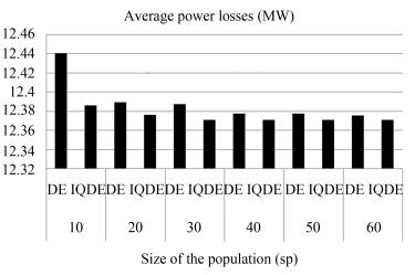
Table Ⅳ Statistics of Results for DE and IQDE (IEEE 14-Bus)

SP	Algorithm	Loss_min	Loss_max	Loss_avg	Time_min	Time_max	Time_avg
10	DE	12.3714	13.1578	12.4401	3.8977	5.3590	4.9267
	IQDE	12.3712	12.5450	12.3858	4.9335	9.0550	7.2024
20	DE	12.3713	12.6364	12.3892	8.7948	9.9069	10.6250
	IQDE	12.3712	12.4035	12.3761	7.8281	14.6796	11.2216
30	DE	12.3712	12.549	12.3876	12.569	15.7014	14.8099
	IQDE	12.3712	12.3712	12.3712	12.1678	17.7190	14.7212
40	DE	12.3712	12.4463	12.3776	16.6632	21.4070	20.2090
	IQDE	12.3712	12.3712	12.3712	15.2144	21.7840	17.3987
50	DE	12.3712	12.4319	12.3774	19.3238	26.4667	25.0056
	IQDE	12.3712	12.3712	12.3712	19.0269	26.7894	22.9460
60	DE	12.3712	12.399	12.3754	25.2242	33.3440	30.3782
	IQDE	12.3712	12.3712	12.3712	24.4536	33.4038	28.0544

下载: 导出CSV

Table Ⅴ Control Variable Setting and P_LOSS Before and After Optimization for IEEE 14-Bus System

	U₁	U₂	U₃	U₆	U₈	T₄	T₅	T₇	Q₉	Q₁₄	P_loss
Before	1.06	1.045	1.01	1.07	1.09	0.978	0.969	0.932	18	18	13.393
After	1.1	1.0779	1.0465	1.1	1.1	1.06	0.9	1.03	18	6	12.3712

下载: 导出CSV

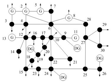
Table Ⅵ Number of Control Variables of IEEE 30-Bus System

Variable	Number
T	4
U	6
Q	2
SUM	12

下载: 导出CSV

Table Ⅶ Setting of Control Variables of IEEE 30-Bus System

Variable	Minimum	Maximum	Step
T	0.9	1.1	0.02
U	0.9	1.1	-
Q₉	0	0.2	0.05
Q₂₄	0	0.04	0.01

下载: 导出CSV

Table Ⅷ Constraints of the State Variables of 30-Bus

Node	Min (MVar)	Max (MVar)
1	0	10
2	-40	50
5	-40	40
8	-10	40
11	-6	24
13	-6	24

下载: 导出CSV

Table Ⅸ Statistics of Results for DE and IQDE (IEEE 14-Bus)

Node	Q_out(MVar)	Q_low	Q_up	P_out (MW)	P_low	P_up
9	0.0137	-0.012	0.025	0.15	0.11	0.19
19	0.0554	-0.013	0.0689	0.25	0.1	0.45
24	0.01	-0.0069	0.02	0.09	0.05	0.15
26	0.0425	-0.15	0.0638	0.185	0.124	0.32

下载: 导出CSV

Table Ⅹ Statistics of Trial Results for IQDE in 30-Bus System Containing DGS

No.	P_loss	Time	No.	P_loss	Time	No.	P_loss	Time
1	16.2163	24.2024	11	16.2163	29.7159	21	16.2164	28.0426
2	16.2163	25.9639	12	16.2163	29.4342	22	16.2163	23.9344
3	16.2164	34.057	13	16.2163	27.2983	23	16.2166	33.3986
4	16.2163	28.0157	14	16.2163	29.5571	24	16.2163	28.6112
5	16.2163	30.1713	15	16.2166	34.6243	25	16.2164	23.7194
6	16.2163	26.3804	16	16.2163	30.1448	26	16.2163	24.2563
7	16.2165	31.7187	17	16.2164	25.1229	27	16.2164	32.3472
8	16.2163	29.4458	18	16.2163	25.7156	28	16.2163	24.8397
9	16.2163	25.2483	19	16.2164	33.2381	29	16.2164	28.5767
10	16.2165	33.7229	20	16.2163	25.9665	30	16.2166	33.8194

下载: 导出CSV

Table Ⅺ Statistics of Trial Results (IEEE 30-Bus)

Results	Average	Min	Max
P_loss	16.2164	16.2163	16.2166
Time	28.7097	23.7194	34.6243

下载: 导出CSV

Table Ⅻ Statistics of Trial Results for IQDE in 30-Bus System Containing DGS

	U₁	U₂	U₅	U₈	U₁₁	U₁₃	T₁₁	T₁₂	T₁₅	T₃₆	Q₁₀	Q₂₄
P₁	1.06	1.045	1.01	1.01	1.082	1.071	1.06	1.04	0.96	1.04	10	3
P₂	1.1	1.0759	1.0431	1.0462	1.1	1.1	0.9	1	1.02	0.9	20	4

下载: 导出CSV

参考文献(18)

[1]	X. Y. Yin, X. Yan, X, Liu, and C. L. Wang, "Reactive power optimization based on improved hybrid genetic algorithm, " J. Northeast Dianli Univ. , vol. 34, no. 3, pp. 48-53, Jun. 2014. http://en.cnki.com.cn/Article_en/CJFDTOTAL-CGCZ201101020.htm
[2]	T. Y. Xiang, Q. S. Zhou, F. P. Li, and Y. Wang, "Research on niche genetic algorithm for Reactive Power Optimization, " Proc. CSEE, vol. 25, no. 17, pp. 48-51, Sep. 2005. http://en.cnki.com.cn/Article_en/CJFDTOTAL-ZGDC200517010.htm
[3]	M. Varadarajan and K. S. Swarup, "Network loss minimization with voltage security using differential evolution, " Electr. Power Syst. Res. , vol. 78, no. 5, pp. 815-823, May2008. http://www.researchgate.net/publication/223544555_Network_loss_minimization_with_voltage_security_using_differential_evolution
[4]	M. Basu, "Optimal power flow with FACTS devices using differential evolution, " Int. J. Electr. Power Energy Syst. , vol. 30, no. 2, pp. 150-156, Jan. 2008. https://www.researchgate.net/publication/222751245_Optimal_power_flow_with_FACTS_devices_using_differential_evolution
[5]	Y. T. Liu, L. Ma, and J. J. Zhang, "GA/SA/TS hybrid algorithms for reactive power optimization, " Proc. the IEEE Power Engineering Society Summer Meeting, Seattle, WA, USA, 2000, 245-249. https://www.researchgate.net/publication/3862451_GASATS_hybrid_algorithms_for_reactive_power_optimization
[6]	B. Zhao, C. X. Guo, and Y. J. Cao, "A multiagent-based particle swarm optimization approach for optimal reactive power dispatch, " IEEE Trans. on Power Syst. , vol. 20, no. 2, pp. 1070-1078, 2005. https://www.researchgate.net/publication/3267300_A_multiagent-based_particle_swarm_optimization_approach_for_optimal_reactive_power_dispatch
[7]	G. F. Fang, H. X. Wang, and X. S. Huang, "An improved genetic algorithm for reactive power optimization, " Proc. the EPSA, vol. 15, no. 4, pp. 15-18, Aug. 2003. http://en.cnki.com.cn/Article_en/CJFDTOTAL-DLZD200304004.htm
[8]	S. F. Wang, Z. P. Wan, H. Fan, C. Y. Xiang, and Y. G. Huang, "Reactive power optimization model and its hybrid algorithm based on bilevel programming, " Power Syst. Technol. , vol. 29, no. 9, pp. 22-25, May. 2005. https://www.researchgate.net/publication/290751059_Reactive_power_optimization_modeland_its_hybrid_algorithm_based_on_bilevel_programming
[9]	W. Liu, X. L. Liang, and X. L. An, "Power system reactive power optimization based on BEMPSO, " Power Syst. Protect. Control, vol. 38, no. 7, pp. 16-21, Apr. 2010. http://en.cnki.com.cn/Article_en/CJFDTOTAL-JDQW201007006.htm
[10]	L. F. Zheng, J. Y. Chen, H. Lin, S. L. Le, and F. Chen, "Reactive power optimization based on quantum particle swarm optimization in electrical power system, " Central China Electr. Power, vol. 24, no. 2, pp. 16-19, 2011. http://en.cnki.com.cn/Article_en/CJFDTOTAL-HZDL201102005.htm
[11]	B. Li, "Research of distribution reactive power optimization based on modified differential evolution algorithm, " M. S. thesis, North China Electr. Power Univ. , Beijing, China, 2012.
[12]	D. Devaraj and J. P. Roselyn, "Genetic algorithm based reactive power dispatch for voltage stability improvement, " Int. J. Electr. Power Energy Syst. , vol. 32, no. 10, pp. 1151-1156, Dec. 2010. https://www.researchgate.net/publication/229092065_Genetic_algorithm_based_reactive_power_dispatch_for_voltage_stability_improvement
[13]	Z. C. Hu, X. F. Wang, and G. Taylor, "Stochastic optimal reactive power dispatch: formulation and solution method, " Int. J. Electr. Power Energy Syst. , vol. 32, no. 6, pp. 615-62, Jul. 2010. https://www.researchgate.net/publication/245214843_Stochastic_optimal_reactive_power_dispatch_Formulation_and_solution_method
[14]	T. Malakar and S. K. Goswami, "Active and reactive dispatch with minimum control movements, " Int. J. Electr. Power Energy Syst, vol. 44, no. 1, pp. 78-87, Jan. 2013. https://www.researchgate.net/publication/256970308_Active_and_reactive_dispatch_with_minimum_control_movements
[15]	R. Storn and K. Price, "Differential evolution-a simple and efficient heuristic for global optimization over continuous spaces, " J. Glob. Optim. , vol. 11, no. 4, pp. 341-359, Dec. 1997.
[16]	W. F. Gao, S. Y. Liu, and L. L. Huang, "A novel artificial bee colony algorithm based on modified search equation and orthogonal learning, " IEEE Trans. Cybernet. , vol. 43, no. 3, pp. 1011-1024, Jun. 2013. https://www.researchgate.net/publication/232533895_A_Novel_Artificial_Bee_Colony_Algorithm_Based_on_Modified_Search_Equation_and_Orthogonal_Learning
[17]	F. S. Abu-Mouti and M. E. El-Hawary, "Optimal distributed generation allocation and sizing in distribution systems via artificial bee colony algorithm, " IEEE Trans. Power Deliv. , vol. 26, no. 4, pp. 2090-2101, Oct. 2011. https://www.researchgate.net/publication/252062867_Optimal_Distributed_Generation_Allocation_and_Sizing_in_Distribution_Systems_via_Artificial_Bee_Colony_Algorithm
[18]	R. W. Keyes, "Quantum computing and digital computing, " IEEE Trans. Electron Devices, vol. 57, no. 8, pp. 2041, Aug. 2010. https://www.researchgate.net/publication/260512239_Quantum_Computing_and_Digital_Computing