Solar thermal power generation system is affected by natural factors such as solar radiation, and also the system has strong interference. These uncertain factors directly affect the quality of solar thermal power generation. Regulating the tracking error of output oil temperature of collector is an important control objective, therefore it has practical significance to study the active fault tolerant predictive control of solar collector system in the state of fault or disturbance.

The solar collector system uses the solar radiation to heat the heat conduction oil, regulates the flow of heat conduction oil, and controls the outlet temperature of the heat conduction oil in a certain range so as to ensure the stability of the power generation. The control objective of the collection system is that the amount of the actual output is as close as possible to the amount of the desired target output. In recent years, many kinds of intelligent control algorithms are applied to the control of solar thermal power generation system [1]-[3]. Reference [4]-[7] all applied the model predictive control algorithm, where the control target was to minimize the tracking error.

Error of the outlet temperature and the single model are used to predict the model. Multi-model adaptive switching active fault tolerant control is about selecting the model with least cumulative error to determine which model of multi-models is the best match for the dynamic behavior of the system online, and continuously optimize the model parameters. The adaptive model which can be reassigned is used to compensate for the missing data in the process of modeling and to reduce the tracking error with strong disturbance or fault conditions. The algorithm has been successfully applied to other areas [8]-[10], the control effect is good. Based on the above analysis, the main research contents of this paper include:

1) Establish multi-model set. Collect data sets for several consecutive days to make the fuzzy C-means (FCM) clustering.

2) Design active fault tolerant sliding mode predictive controller. Determine the adaptive switching strategy. The inlet temperature and solar radiation are considered as disturbance, and flow of heat conduction oil is considered as controlled variable. Based on the multi-model, the adaptive model of the solar collector system is established to adapt the object and the disturbance characteristics. A model switching strategy based on the minimum cumulative error is used to select the optimal control model online.

3) The method is applied to the actual linear Fresnel power generation system, and the method is compared with [3]. The method in this paper is better than the method [3], the control precision is higher, and the time delay is shorter.

1.   Dynamic Model of Solar Thermal Power Generation System

1.1   The Mathematical Model of Micro-sources

1.1.1   Microturbine Cost

R Carmona, a Spanish scholar, initially used the mathematical model [1] to describe the temperature of heat conduction oil of the solar collector [11], and then the model was used to analyze the thermal system [4]-[6].

where $t$ is time, s; $\Delta x$ is length of the collector tube section; ${\rho _{\rm{f}}}$ is refrigerant density, kg/m $^3$ ; ${C_{\rm{f}}}$ is specific heat capacity, ; ${A_{\rm{f}}}$ is cross section area of pipe; $v(t)$ is conduction heat oil flow, ${\rm m^3}$ /s; $I(t)$ is solar intensity, W/ ${\rm m^2}$ ; ${\rm \eta _0}$ is mirror optical efficiency; ${G_1}$ is the optical aperture of reflector, m; $Tn$ is conduction heat oil temperature of oil pipeline outlet, ℃; $Tn - 1$ is conduction heat oil temperature of oil pipeline outlet, ℃.

Take $\Delta x$ = $L$ , then (1) can be

where $L$ is the total length of pipeline of the collection system; $T{}_0(t)$ is the entrance conduction heat oil temperature of collector.

2.   Clustering Modeling of Solar Thermal Power Generation Set

2.1   Fuzzy Clustering of Data Set

The data acquisition in the linear Fresnel thermal power generation system is used to make FCM clustering analysis. In this clustering algorithm, the membership degree is used to determine the degree of each element and the measured data is classified by the method of subtraction clustering [12], [13].

Step 1: Determine the number of categories $C$ , fuzzy weight index m and the initial clustering center $v$ ;

Step 2: The fuzzy membership degree ${u_{ij}}$ is calculated according to

${u_{ij}}$ is the fuzzy membership degree of category $J$ of individual. ${\upsilon _j}$ is cluster center of category $J$ .

Step 3: Use (4) to calculate the center of each category.

Step 4: The target value is calculated according to (5) to determine whether the values meet the target value or not. If the values meet the target value, the clustering is end. Otherwise, return Step 2.

In this paper, DB is used as an evaluation index of the classification [14]. The smaller the index value is, the better the clustering effect is. In this paper, for 3500 sets of actual power generation data $M$ from the solar thermal power generation system of Gansu Lanzhou Dacheng company, which is put into use in Lanzhou New District, $M({m_1}$ , ${m_2}$ , ${m_3}$ , ${m_4}$ ) is classified, among them, ${m_1}$ is the outlet temperature, ${m_2}$ is the heat transfer oil outlet temperature, ${m_3}$ is flow, and the solar radiation is ${m_4}$ . Fuzzy clustering is used to analyze such data. When $C$ = 6, DB is the smallest, and Table Ⅰ lists the clustering results.

表 Ⅰ  Clustering Results

Table Ⅰ  Clustering Results

C	2	3	4	5	6	7	8	9
DB	1.3893	1.0168	0.6306	0.7065	0.1746	0.9135	0.4936	0.6304

下载: 导出CSV 

| 显示表格

The clustering centers of the 6 types are respectively:

2.2   Least-squares Modeling

The above classification data results considered the inlet oil temperature, solar radiation and flow rate of conduction heat oil as input, and outlet temperature as output. In order to overcome the shortcomings of the least squares due to its poor correction ability, forgetting factor recursive least square method is adopted [9], [15], [16]. The controlled auto regressive (CAR) model expressed by formula (6) is used to identify the parameters.

where,

Initial value $\theta (0) = 0$ is the positive real vector with zero or small value. The mathematical model of the solar collector system can be obtained, as shown in the model (7).

where ${y_i}(k)$ is output oil temperature, ${u_i}(k)$ is the flow rate of conduction heat oil, ${T_{\rm in}}_{ i}(k)$ is input oil temperature, and ${I_i}(k)$ is solar radiation.

According to the results of the optimal clustering center, the outlet temperature is considered as the center to analyze the error of classification. Fig. 1 shows the effect of deviation of each class of data from the center point of the cluster. In different temperature and cross sectional output data, outlet temperature is also affected by the inlet temperature and solar radiation. Therefore, the system can be considered as a multi disturbance system.

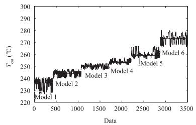图 1  Error of multi-model and clustering center.

Fig. 1  Error of multi-model and clustering center.

下载: 全尺寸图片 幻灯片

3.   Multi-model Active Fault Tolerant Sliding Mode Predictive Controller

Predictive control includes prediction model, rolling optimization and feedback correction. Under the condition of system fault or disturbance, the multi-model adaptive switching active fault tolerant control can update the control law based on the optimal predictive model online, which results in stable operation of the closed-loop system. In the process of rolling optimization, update control law online, and through the feedback of correction, the error is corrected online. Fig. 2 is the structure of a multi-model active fault tolerant controller of solar thermal power generation. ${y_r}(k)$ is the desired output, $y(k)$ is the actual output of model, ${y_i}(k)$ is the most optimal sub model, and ${y_p}(k)$ is the adaptive model.

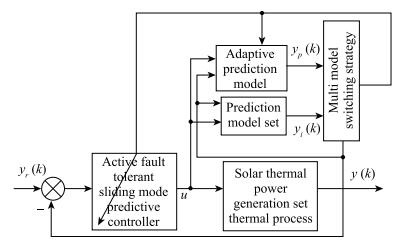图 2  The structure of a multi-model active fault tolerant controller of solar thermal power generation.

Fig. 2  The structure of a multi-model active fault tolerant controller of solar thermal power generation.

下载: 全尺寸图片 幻灯片

In [17]-[19], a single model sliding mode predictive control is designed for the high speed aircraft. In [18], a multi-model sliding mode predictive control is designed for the disturbance signal. Active fault tolerant predictive controller is designed for high-speed train based on [19]. In the literature, the designed controller according to different system has achieved good control effect. By referring to the above documents, this article designed the active fault tolerant control in solar thermal applications. Consider the following uncertain discrete linear systems

where $y(k)$ is the output, $u(k)$ $\in \mathbb{R}$ is the control input, $A$ and $B$ are matrixes with appropriate dimension, and is the total interference.

3.1   Sliding Mode Surface Design

Define the switching function: set the reference command signal ${y_r}(k)$ , define the tracking error (9).

Define the linear switching function:

where ${\sigma ^{T}} = [{\sigma _1}, \ldots, {\sigma _n}]$ . After the solar collector model expression (2) is discretized, the configuration of poles of the expected oil outlet temperature is set inside the unit circle, and then ${\sigma _i}$ is obtained through the calculation. In order to guarantee the stability and dynamic performance of the ideal sliding mode, construct the following sliding mode prediction model.

The predicted sliding mode surface is ${S_m} = \{ e(k)|{s(e(k))}$ $=$ $0\}$ . The p step ahead predictor is as follow.

Use the difference value between actual switching function output value $s(k)$ and $p$ step ahead prediction at the moment of $k - p$ to make the feedback correction of output value ${s_p}(k + p)$ of sliding mode prediction model. Thus, the output of the closed-loop sliding mode prediction model can be expressed as:

where ${\zeta _p} \in \mathbb{R}$ is the weighted feedback correction factor. Let ${\zeta _1}$ $=$ $1$ , $0 < {\zeta _p} < 1$ $(p \ge 1)$ . Decrease of ${\zeta _p}$ can reduce the role of feedback correction.

3.2   Sliding Mode Reference Trajectory

Take the commonly reaching rate as the reference trajectory.

where $0 < \mu < 1, $ $\eta >0$ . The greater the $\mu $ , the smaller the switching power. Control objective is that the error state reaches the sliding mode surface that is to say $s(e(k)) = 0$ .

3.3   Control Law Design

Define the performance index

where $N$ and $M$ are positive integers, which respectively represent the predicted time domain and control time domain, $M$ needs to meet $N< 0 < M, $ $u(k + j) = u(k + M - 1)$ , $M $ $\le$ $j$ $<$ $ N$ , and ${\lambda _j}$ is weight coefficient.

If the output vector is expressed as:

then (12) and (13) can be represented as a vector form, which can be expressed by (16) and (17).

So, the performance index expressed by(15) can be written as a vector form expressed by (18).

where ${L_0}=$ $[1, $ $\ldots, 1]^{T}, $ ${L_1} = {[{\gamma ^1}, \ldots, {\gamma ^N}]^{T}}, $ $ 0 $ $< \gamma$ $<$ $1, $ .

Let $\frac{{\partial J(U)}}{{\partial U}} = 0$ , solve the corresponding equations, and the optimal flow rate of $U$ in the collection process is calculated:

3.4   Multi-model Switching Strategy

The switching strategy is to select the optimal control model online [18] for the state of system under the condition of unknown fault or disturbance, and the active fault tolerant predictive control is carried out through the rolling optimization and feedback correction.

At the $k$ th moment, ${e_i}(k) = y(k) - {\hat y_i}(k)$ is the output error between actual output and $i$ $(1 \le i \le P* + 2)$ model. The definition of switching index is shown in (20).

where $\alpha $ is error coefficient at present, $\beta $ error coefficient for historical moment, $\alpha > 0, $ $\beta > 0, $ $\alpha + \beta = 1$ , $L$ is the number of the concerned historical sampled data, and $\theta = 1$ .

3.5   Adaptive Fault-tolerant Control

3.5.1   Active Fault-tolerant Algorithm

Under the condition of system failure or disturbance, the active fault tolerant control can update the control law according to the optimal control model online selection, which can stabilize the closed loop system [19]. Active fault tolerant control is realized by the adaptive model switching.

3.5.2   Adaptive Model Switching

The adaptive model can be used to obtain a faster convergence rate according to the different conditions. According to the model switching strategy, if the initial parameters of the model are the optimal model parameters of the multi-model set, the optimal model can be selected from the current optimal model set and the parameters can be updated with (21). Otherwise, the initial value of the model is reassigned to the minimum cumulative error model parameters, and then the model parameters are updated online through (21). According to the model switching strategy, the obtained optimal model is the adaptive model, which can guarantee the stability of the system and the accuracy of tracking. Parameters are updated as follows [9], [19].

where $\theta (k)$ are the parameters to be identified, $K(k)$ is gain matrix, $\varphi (k)$ is observation matrix, $P(k)$ is covariance matrix, and $\lambda $ is forgetting factor.

4.   Simulation Result Analysis

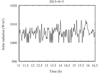
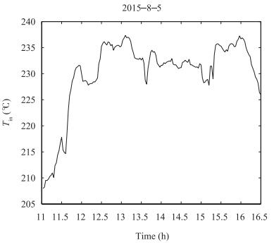
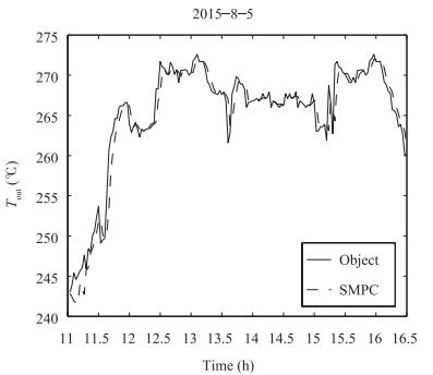
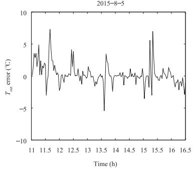
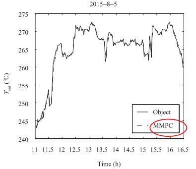
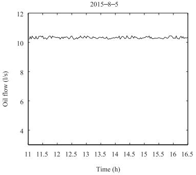
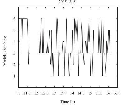
In the process of simulation analysis, system model selects (2). Parameters of the linear Fresnel power generation demonstration project in the west of China are selected and the outlet oil temperature of conducting oil on August 5, 2015 is taken as the target curve. Controlled variable is the flow of heat conduction oil. Inlet oil temperature and solar radiation are disturbances which can be measured. The flow range of heat conduction oil is 3 (l/s)-12 (l/s). ${\eta _0} = 0.60, $ ${C_f}$ $=$ $2600 {\rm J/kg}{^\circ}{\rm C}, $ $T = 20$ s, $L = 220$ m, m $^2$ , $G$ $=$ $0.80$ m. Parameter values of simulation analysis are: $\alpha$ $=$ $0.3, $ $\beta = 0.7$ , $\theta $ is the positive real vector with zero or small initial value, , and forgetting factor $\lambda $ $=$ $0.95$ . Methods in [3] are compared with this paper, the two algorithms simulation results are shown in Fig. 3 to Fig. 8. Fig. 7 and Fig. 10 are the flow of heat conductive oil, and the curve of the control value respectively. Fig. 11 is switching progress between the six models.

图 3  Solar radiation intensity.

Fig. 3  Solar radiation intensity.

下载: 全尺寸图片 幻灯片

图 4  Inlet oil temperature.

Fig. 4  Inlet oil temperature.

下载: 全尺寸图片 幻灯片

图 5  Control efiect of [3].

Fig. 5  Control efiect of [3].

下载: 全尺寸图片 幻灯片

图 6  Tracking error of [3].

Fig. 6  Tracking error of [3].

下载: 全尺寸图片 幻灯片

图 7  Oil flow of [3].

Fig. 7  Oil flow of [3].

下载: 全尺寸图片 幻灯片

图 8  Control efiect of this paper.

Fig. 8  Control efiect of this paper.

下载: 全尺寸图片 幻灯片

图 9  Output error of this paper.

Fig. 9  Output error of this paper.

下载: 全尺寸图片 幻灯片

图 10  Oil flow result of this paper.

Fig. 10  Oil flow result of this paper.

下载: 全尺寸图片 幻灯片

图 11  Curve of models switching.

Fig. 11  Curve of models switching.

下载: 全尺寸图片 幻灯片

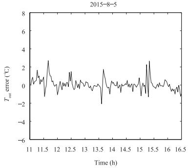
The average variance of two kinds of simulation results is analyzed and calculated. MSE = 1.53264 in Fig. 5 and MSE = 0.43276 in Fig. 8.

It can be seen from Fig. 7 and Fig. 10 that multi-model active fault-tolerant sliding mode predictive control is better than that of [3].

5.   Conclusion

In this paper, we collected the data of 3500 sets of solar thermal power generation sets, classified them, and set up the mathematical model. A fault-tolerant sliding mode predictive controller is designed, which can reduce error, improve the system's robustness and anti-interference ability. The adaptive prediction model can be used to reduce the error caused by loss of data, the disturbance and fault.

From Fig. 5 and Fig. 8, it can be seen that the method proposed in this paper has higher accuracy and shorter lag time, and has the ability to improve the robustness and convergence rate of the solar thermal power generation system.