1.   Introduction

With the increasingly complicated engineering problems during the past few years, many researchers devote themselves to researching new intelligent optimization algorithms. In 2011, a new heuristic optimization algorithm named fruit fly optimization algorithm (FOA) is proposed by Pan [1] who is inspired by the feeding behaviors of drosophila. FOA is easy to be understood, and it can deal with the optimization problems with fast speed and high accuracy, while, the results are influenced a lot by the initial solutions [2]. Based on the phototropic growth characteristics of plants, a new global optimization algorithm called plant growth simulation algorithm is proposed by Li et al., which is a kind of bionic random algorithm and suitable for large-scale, multi-modal and nonlinear integer programming [3], however, for its complex calculation theory, the algorithm is not widely applied in industry and scientific research. Artificial bee colony algorithm [4] is a new application of swarm intelligence, which simulates the social behaviors of bees, whose defects are slow convergence speed and easy to trap into local optimum [5].

Mirror is a common necessity, which plays an important role in daily life. Inspired by the optical function of mirror, a new algorithm called specular reflection algorithm (SRA) is raised by this paper. SRA, similar to genetic algorithm [6]-[8], particle swarm optimization [9]-[11], simulated annealing algorithm [12], [13], differential evolution algorithm [14], [15], etc, can be widely used in science and engineering. The SRA has many outstanding advantages, such as simple principle, easy programming, high precision and fast calculation speed, and its unique non-population searching mode distinguishes itself from original swarm algorithm. Furthermore, the global searching ability is significantly improved by the specific acceptance criterion of the new solution. In order to verify above mentioned features of SRA, a great deal of comparative experiments are adopted in this paper. At last, the reliability based design and robust design are combined with the SRA, in order to evaluate the ability of SRA in reliability based robust optimization design.

2.   SRA

2.1   Introduction of SRA

Mirror is a life necessity and a product of human civilization, which can change the direction of propagation of light. There are various kinds of mirrors, such as magnifying glass, microscope, etc. With the help of mirror, a great deal of stuff can be observed, even if they are out of the range of visibility. For example, the submarine soldier is able to catch sight of the object above the water by periscope. This reflection property of mirror is simulated by the SRA.

Object, suspected target, eyes and mirror are the four basic elements of specular reflection system.

Object is the objective function of optimization. Getting its exact coordinate is the purpose of the SRA. It is not involved in the optimization procedure for the location of the object is unpredictable.

Suspected target is the coordinate of the object observed by eyes, which is approximate to the optimal solution. There is an error between the suspected target and object, because the coordinate of the object observed by eyes is not accurate. The suspected target is located around the object, and it is the element nearest to the object.

Mirror can change the direction of propagation of light. The vision of eyes can be broaden by mirror. All the things that can reflect light (glass, water, etc.) are taken as mirror.

Eyes are the subject of the SRA, which can acquire the approximate coordinate of the object. And it is the element farthest from the object.

2.2   Definition

Taking the constrained optimization problem showed in (1) as an example, the definition of SRA will be drawn as following:

Set the specular reflection system as a $ 4\times N$ dimensional Euclidean space, where $N$ is the number of design variables. The elements in the system are defined as $X_i$ , $x_i^N)$ , $i = (0, 1, 2, 3)$ , and , $X_{\rm Suspect} = X_1$ , $X_{\rm Mirror}$ $=$ $X_2$ , . Where $x_i^n$ $(n=1, 2, \ldots, N)$ is the position of the $i$ th variable in the $N$ dimensional space. The four elements of SRA can be defined as $f(X_i)$ , and the relationship among the four elements is $f(X_0)\leq f(X_1) \leq$ $f(X_2)$ $\leq$ $f(X_3)$ .

Searching the new coordinate: the coordinates of $X_{\rm New1}$ and $X_{\rm New2}$ can be acquired by (2), and the new coordinate of $X_{\rm New}$ can be got by (2).

where $\xi$ is coefficient, which is determined by (11).

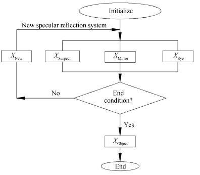
Updating the specular reflection system: Once the coordinate of $X_{\rm New}$ is acquired, the eyes will change its place to continue searching for the "object", the four elements of the system are $X_0 X_1 X_2$ and $X_{\rm New}$ under the current situation. The specular reflection system will be adjusted by the modification of the four elements, the system will be changed by the rules shown in Fig. 1.

图 1  Coordinate update of the specular reflection system.

Fig. 1  Coordinate update of the specular reflection system.

下载: 全尺寸图片 幻灯片

The optimization steps of the SRA are shown as follows:

Step 1: Define the initial value $X_i$ , $i = 0, 1, 2, 3$ , and the maximum iteration number $Iter_{\max}$ .

Step 2: If the precision or the maximum iteration number reaches the design requirements, the coordinate of $X_{\rm Object}$ will be output which is the optimum solution. Otherwise, execute the next step continually.

Step 3: Search the coordinate of $X_{\rm New}$ by (2) and (3), the new iteration process will begin, then go back to Step 2 and Continue to calculate.

In conclusion, the optimization flow chart of the SRA is given by Fig. 2.

图 2  Optimization flow chart of the SRA.

Fig. 2  Optimization flow chart of the SRA.

下载: 全尺寸图片 幻灯片

2.3   Optimization Flow Chart of the SRA

Theorem 1: The constraint optimization problem presented in (1) can converge to the global extremum with 100 % probability by the SRA.

Proof: Provided that $X_{\rm Object} = \min f(X)$ , $X\in D$ which is the global optimal solution, where $f(X_{\rm Object})$ is the optimal value of objective function, $D$ is the feasible region and $D=\{X|g_j (X_{\rm Object}) = 0$ , $j = 1, 2, \ldots, m$ ; , $k$ $=$ $1$ , $2$ , $\ldots$ , $l$ ; and $D\in \mathbb{R}^N$ .

First, get the feasible initial solutions $X_{\rm Suspect}^0$ , $X_{\rm Mirror}^0$ and $X_{\rm Eyes}^0$ randomly among the searching space, where $X_{\rm Suspect}^0$ , $X_{\rm Mirror}^0$ , , and the corresponding values of objective function $f (X_{\rm Suspect}^0)$ , $f(X_{\rm Mirror}^0)$ and $f(X_{\rm Eyes}^0)$ can be worked out, where $f(X_{\rm Mirror}^0)$ $\leq$ $f(X_{\rm Eyes}^0)$ .

Second, the new solutions $f(X_{\rm Suspect}^k)$ , and $f(X_{\rm Eyes}^k)$ can be acquired according to the new specular reflection system, where are the randomly produced solutions which are uniformly distributed in , $X_{\rm Suspect}^k$ is the solution of the $k$ th ( iteration, $X_{\min}^k$ and $X_{\max}^k$ are the boundaries of design variable in the current iteration, and the maximum iteration number $Iter_{\max}$ should be big enough. Therefore, under the uniform distribution, the probability of generating the feasible solutions is:

where $\varepsilon$ is a real number which is sufficiently small; $X_{\rm max}$ and $X_{\rm min}$ are the extreme values of the 4 $\times N$ dimensional Euclidean space.

The probability that the feasible solution $X_{\rm Suspect}^0$ is optimal is $P^1$ , and the probability that $X_{\rm Suspect}^0$ is not optimal is $Q^1$ , both $P^1$ and $Q^1$ are expressed as follows:

where $X_{\rm Suspect}^0$ is the feasible solution gotten for the first time.

The probability that the feasible solution gotten for the second time still failing to be the optimal value is:

So, the probability that the solution is optimal is:

After $n$ times iteration, the probability of getting the optimum solution can be acquired by the following inference.

Calculate the extreme value of (8):

With the iterations going on, it is more and more likely to achieve the optimum solution. When $n\rightarrow \infty$ , , it indicates that the searching process of SRA can converge to the global extreme with 100 % probability.

2.4   Selection of Control Parameter

The control parameter is closely related to the space complexity of optimized target, which has an effect on the capability of algorithm. The control parameters of classical optimization algorithm are gotten by experience or experiment, such as the learning parameter $c_1 = c_2$ = 2 by PSO [16], [17], and the crossover probability and mutation probability of GA [18]. It is impossible that the control parameter acquired by experience is suitable for all optimization problems. The SRA only has the control parameter $\xi$ , whose value will have a prominent effect on SRA. In this section, a classical test function is used to confirm the most appropriate value of $\xi$ , and the results are listed in Table Ⅰ.

表 Ⅰ  JUDGEMENT OF $\xi$

Table Ⅰ  JUDGEMENT OF $\xi$

Value of $\xi$	N =2		N =10		N=20		N=50		N = 100
	Optimal solution (10-6)	Iteration times	Optimal solution (10-6)	Iteration times	Optimal solution (10-6)	Optimal solution (103)	Optimal solution (10-6)	Optimal solution (103)	Optimal solution (10-6)	Optimal solution (104)
0.4	4.7776	402.70	7.1895	1103	7.2883	2.0369	8.9324	6.1015	9.5844	1.4945
0.5	3.3845	341.04	6.4267	940.12	7.3111	1.8001	8.4771	5.3149	9.6383	1.2586
0.6	3.9884	737.76	5.4844	936.46	7.2327	1.6802	9.0155	4.8292	9.3691	1.1344
0.7	3.5625	515.18	6.9587	810.24	7.2858	1.5971	8.5419	4.4544	9.5971	1.0679
0.8	4.2770	509.46	6.7379	747.90	7.5046	1.4992	8.8811	4.2697	9.3384	1.0741
0.9	4.0589	259.08	6.3850	732.90	7.4304	1.4562	8.3421	4.2036	9.4009	1.0976
1.0	4.9287	193.26	5.9257	694.18	6.8977	1.3677	8.3414	4.3603	9.5947	1.1404
1.1	4.6702	142.60	6.1496	674.28	8.0852	1.2946	9.4538	4.2854	9.4944	1.1889
1.2	4.6250	142.42	5.8875	626.54	7.7654	1.3608	8.6969	4.4775	9.6771	1.2434
1.3	5.1501	139.08	6.5208	654.72	7.2172	1.4050	8.9588	4.5342	9.5792	1.3215
1.4	5.4409	131.02	5.6072	695.40	6.9556	1.4699	8.9053	4.6930	9.6898	1.3675
1.5	4.7099	103.72	5.7050	675.02	7.6612	1.4740	9.0472	4.8329	9.5134	1.4173
1.6	4.7625	93.82	5.8038	713.20	6.4546	1470	8.9756	4.8634	9.7748	1.4768
1.7	4.9327	91.94	4.9871	783.90	5.8034	1.6036	9.1825	5.0851	9.6612	1.4985
1.8	5.9076	87.32	5.4104	856.30	7.1143	1.6917	8.7372	5.3202	9.4446	1.5536
1.9	4.9402	82.44	5.5724	832.12	6.4092	1.8641	8.7754	5.5962	9.6617	1.6423
2.0	4.7168	89.08	4.8307	998.300	5.7508	2.0544	8.1780	6.3700	9.4975	2.5117

下载: 导出CSV 

| 显示表格

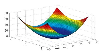
The test function is illustrated by (10), and its three-dimension diagram is shown in Fig. 3. The global minimum value in theory of this function is 0 $(0, 0, \ldots, 0)$ and the constraint condition is $-5.12\leq x_j\leq 5.12$ , $j=1, 2, \ldots, N$ . In consideration of $N = (2, 10, 20, 50, 100, 500)$ and $\xi = (0.4$ , $0.5$ , $\ldots$ , $2.0)$ , do the calculation 50 times using every possible combination of $N$ and $\xi$ , then put the average results in Table Ⅰ. Assume that the convergence condition is $Iter_{\max}$ $=$ $10^5$ or $f (x_1, x_2, \ldots, x_N )\leq 10^{-5}$ .

图 3  Three-dimensional surface of test function.

Fig. 3  Three-dimensional surface of test function.

下载: 全尺寸图片 幻灯片

As shown in Table Ⅰ, all the results fall in between 10 $^{-5}$ and 10 $^{-6}$ , the optimization efficiency which is influenced by $\xi$ cannot be evaluated by the optimal solutions, therefore, iteration times is the only factor to be considered.

According to the Table Ⅰ, the conclusions can be drawn as follows: when $N = 2$ and $\xi = 1.9$ , the efficiency of the optimization is highest, the corresponding iteration is 82.44; When $N = 10$ , , $N = 50$ and $N = 100$ , the best $\xi$ and its corresponding iteration times are 1.3 and 654.72, 1.1 and $1.2946\times 10^3$ , 0.9 and $4.2036\times 10^3$ , 0.7 and $1.0679$ $\times$ $10^4$ , respectively. In addition, the value of $\xi$ will be reduced gradually with the increasing of $N$ , and the relationship between $\xi$ and $N$ (as shown in (11)) can be speculated by the method of data fitting.

2.5   Simulation Experiments

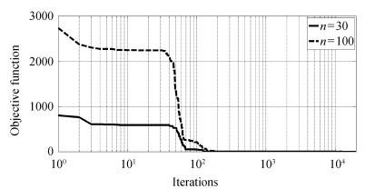
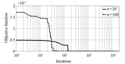
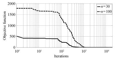
To verify the global optimization ability of SRA, four numerical test functions in [10] are used, each test function is listed in Table Ⅱ in detail. The total iteration time is set as 2000. The SRA will be executed 50 times, and the average values are listed in Table Ⅲ, other results are references from [10], Figs. 4-7 show the iteration curves of the objective functions of each test function respectively.

表 Ⅱ  NUMERICAL CALCULATION FUNCTION

Table Ⅱ  NUMERICAL CALCULATION FUNCTION

Name	Expression	Interval of convergence	Global extreme	Dimension
Sphere	$f_1 = \sum\limits_{i = 1}^n {x_i^2 }$	$x_i\in [-50,50]$	0 (0, 0, $\ldots$ , 0)	$n$ = 30 100
Griewank	$f_2 = 1 + \sum\limits_{i = 1}^n {\left( {\frac{x_i^2 }{4000}} \right) -\prod\limits_{i = 1}^n {\cos \left( {\frac{x_i }{\sqrt i }} \right)} }$	$x_i\in [-600,600]$	0 (0, 0, $\ldots$ , 0)	$n$ = 30 100
Rosenbrock	$f_3 = \sum\limits_{i = 1}^{n - 1} {[100(x_{i + 1}-x_i^2 )^2 + (x_i-1)^2]}$	$x_i\in [-100,100]$	0 (1, 1, $\ldots$ , 1)	$n$ = 30 100
Restrigin	$f_4 = \sum\limits_{i = 1}^n {[10 + x_i^2-10\cos (2\pi x_i )]}$	$x_i\in [-5.0, 5.0]$	0 (0, 0, $\ldots$ , 0)	$n$ = 30 100

下载: 导出CSV 

| 显示表格

表 Ⅲ  CALCULATION RESULTS OF TEST FUNCTION

Table Ⅲ  CALCULATION RESULTS OF TEST FUNCTION

Name	PSO (n = 30) [10]	Kalman swarm (n = 30) [10]	Chaos ant colony optimization (n = 30)[10]	Chaos PSO (n = 30) [10]	New chaos PSO (n = 30) [10]	SRA (n = 30)	SRA (n = 100)
Sphere	3.7004×102	4.723	3.815×10-1	2.4736×10-3	2.0729×10-9	1.1080×10-24	2.3160×10-12
Griewank	2.61×107	3.28×103	23.414	6.8481×10-2	9.9051×10-11	4.6629×10-15	2.7978×10-14
Rosenbrock	13.865	9.96×10-1	4.669×10-1	1.0404×10-2	2.9068×10-4	9.8730×10-7	6.1173×10-5
Restrigin	1.0655×102	53.293	22.6361	9.5258×10-1	4.3741×10-4	3.9373×10-21	8.7727×10-7

下载: 导出CSV 

| 显示表格

图 4  Iteration curve of sphere.

Fig. 4  Iteration curve of sphere.

下载: 全尺寸图片 幻灯片

图 5  Iteration curve of griewank.

Fig. 5  Iteration curve of griewank.

下载: 全尺寸图片 幻灯片

图 6  Iteration curve of rosenbrock.

Fig. 6  Iteration curve of rosenbrock.

下载: 全尺寸图片 幻灯片

图 7  Iteration curve of restrigin.

Fig. 7  Iteration curve of restrigin.

下载: 全尺寸图片 幻灯片

The results in Table Ⅳ indicate that: when $n$ = 30, the results of the four test functions calculated by SRA are , $4.6629 \times 10^{-15}$ , $9.8730 \times 10^{-7}$ and $3.9373$ $\times$ $10^{-21}$ respectively, which are , $2.12 \times 10 ^4$ , $2.90$ $\times$ $10^2$ , times higher than the results gotten by new chaos PSO algorithm which possesses the highest accuracy in [10]; When , the results of the four test functions calculated by SRA are $2.3160\times 10^{-12}$ , $2.7978$ $\times$ $10^{-14}$ , $6.1173\times10^{-5}$ , $8.7727\times 10^{-7}$ respectively, and the computational accuracy are still $8.95\times 10^2$ , , $4.75$ , $4.99$ $\times$ $10^2$ times higher than the results calculated by new chaos PSO algorithm. All in all, the SRA is an efficient optimization algorithm.

表 Ⅳ  CALCULATION RESULTS

Table Ⅳ  CALCULATION RESULTS

Design method		Design variables (mm)					Objective function (mm2)	Reliability	Sensitivity of reliability/(10-3)
		x1	x2	x3	x4	x5	A	Rv	$\frac{\partial R_v}{\partial S}$		$\frac{\partial R_v}{\partial E}$	$\frac{\partial R_v}{\partial \rho}$
SRA	Optimization	6	6	205	635	257	10 704	0.5071	14.3985	0.0017	9.15×10-9	0.0011
	Reliability Optimization	6	6	258	632	310	11 304	0.9968	13.0816	0.0015	8.77×10-9	0.0010
	Robust Reliability Optimization	6	6	324	595	376	11 652	0.9813	12.6270	0.0015	9.23×10-9	0.0010
PSO	Optimization	10	6	185	567	619	11 544	0.5314	13.0714	0.0015	9.8×10-9	0.0010
	Reliability Optimization	7	7	222	605	276	12 334	0.9806	12.9119	0.0015	9.73×10-9	0.0011
	Robust Reliability Optimization	9	6	302	534	354	12 780	0.9810	11.5262	0.0013	1.01×10-8	0.0010
FOA	Optimization	9	6	190	581	633	11 328	0.5132	13.3500	0.0016	9.64×10-9	0.0010
	Reliability Optimization	6	6	491	532	543	13 068	0.9802	11.3697	0.0013	1.01×10-8	9.95×10-4
	Robust Reliability Optimization	8	11	237	536	299	16 576	1.0	11.6479	0.0013	1.27×10-9	0.0013
Note: The index of reliability R0 = 0.98 is deflned.

下载: 导出CSV 

| 显示表格

3.   Reliability Robust Optimization Design

3.1   Reliability Design

According to the reliability design theory, the reliability can be calculated by (12):

where $f_x (X)$ is the joint probability density of basic random variables $X=(X_1, X_2, \ldots, X_n)^T$ , which shows the state of the components.

The basic random variables $X_i$ ( $i = 1, 2, \ldots, n$ ) are independent of each other and follow certain distribution. The reliability index $\beta$ and the reliability $R=\Phi(\cdot)$ can be calculated by Monte Carlo method [19], where $\Phi(\cdot)$ is the standard normal distribution function.

3.2   Reliability Robust Optimization Design

Robust design is a modern design technique that can improve the efficiency and quality and reduce the cost of products [20], [21]. The robust design of mechanical products can make the products insensitive to the changes of design parameters. The product which is designed by robust design method has the characteristic of stability. Even if there is an error in the designed parameters, the product still has excellent performance. Reliability is a kind of design method to eliminate the weaknesses, failure modes and guard against malfunction. The reliability robust optimization design is a new method by combining the robust design and reliability design, which possess all the merits of the two methods. The products designed by the reliability robust optimization design method are reliable and have robustness.

where $f_1(X)$ and $f_2(X)$ are the objective functions of the Reliability Robust Optimization design, $f_1(X)=R$ and $f_2(X)$ is the design criterion related to robust design which can be acquired by (15); $R$ is the reliability; $R_0$ is the constraint condition of reliability; $p_i$ and $q_j$ are equality and inequality constraints of the robust reliability optimization design respectively.

where $\omega_1$ and $\omega_2$ are weighting coefficients, which are related to the importance of $f_1(X)$ and $f_2(X)$ , both of them are calculated by (16), and $\omega_1+\omega_2 = 1$ .

where $X^{1*}$ and $X^{2*}$ are the best values when $\min f(X)$ $=$ $f_1 (X)$ and $\min f(X)=f_2 (X)$ respectively.

4.   Engineering Example

The bridge crane is taken as an example to verify the capability of the SRA in solving the engineering problems. The SRA is adopted to design the structure with optimized design, reliability optimization design and robust reliability optimization design, and the results are listed in Table Ⅲ together with the results calculated by PSO and FOA, which are used for analysing the performance of the SRA.

4.1   Design Parameters

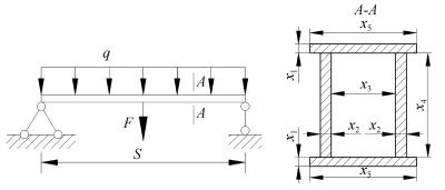
The mechanical model of the bridge crane is shown in Fig. 8, the uniform load $q$ and the concentrated load $F$ are exerted on the girder, where $q$ is caused by the structure deadweight and $F$ is related to the weight of the hoisted cargo.

图 8  Mechanical model diagram and sectional dimension.

Fig. 8  Mechanical model diagram and sectional dimension.

下载: 全尺寸图片 幻灯片

The parameters $x_i$ $(i = 1, 2, 3, 4, 5)$ are considered to be the design variables, where $6\leq x_1$ , $x_2\leq 30$ , $50\leq x_3$ , $x_4$ $\leq$ $5000$ , $x_5 = x_3 + 2x_2 + 40$ . The parameter $S$ is the span of the bridge crane. Other parameters include the elasticity modulus $E$ , the material density $\rho$ , $q$ $=$ $g(x_1$ , $x_2$ , $x_3$ , $x_4, x_5)$ . The parameters $S$ , $F$ , $E$ and $\rho$ are independent of each other, and they are normal random variables, $S$ $\sim$ ${\rm N}(12, 0.08^2)$ , $F$ $\sim$ , $E$ $\sim$ ${\rm N}(206 000$ , $6180^2)$ , $\rho\sim {\rm N}(7850, 5.6^2)$ .

4.2   Optimization Design

Objective function: According to the characteristics of the structural optimization problem, the objective function can be defined as shown in (17).

Constraint condition: Strength, stiffness and stability are the three basic failure modes of bridge crane. Therefore, the constraint condition can be defined as following:

1) Strength Constraint: The maximum stress of dangerous point in mid-span section must be smaller than the ultimate stress $f_{rd}$ ;

where $f_{rd}$ is determined by the limit state method, and $f_{rd}$ $=$ ${f_{yk}}/{\gamma_m} = {235}/{1.1}=213.64$ MPa, $f_{(yk)}$ = 235 is yield stress, $\gamma_m$ = 1.1 is the resistance coefficient, $I_Z$ is moment of inertia of Section 2.1, $q$ and $I_Z$ are the functions related to design variables $x_i$ ( $i$ = 1, 2, 3, 4, 5).

2) Stiffness Constraint: The maximum deflection of the structure must be smaller than the allowable value $\gamma_0$ $=$ $S/400$ .

3) Stability Constraint: The depth-width ratio of Section 2.1 must be smaller than 3.

In conclusion, the optimization model of the bridge crane can be built as (21).

4.3   Reliability Optimization Design

The reliability constraint of structure is added to (21) to achieve the reliability optimization design. The failure of any mode will result in the failure of the structure, so the reliability $R_v$ is defined by (22). The reliability optimization model of bridge crane can be established by (23).

where $R_k$ , $k=1, 2, 3$ is the probability of the $k$ th failure mode.

4.4   Robust Reliability Optimization Design

According to the robust reliability optimization design model which is shown in (14), the index of reliability and robustness are taken into account, the multi-objective optimization model is built by (24).

where .

4.5   Calculation Results

The three optimization models shown in (21), (23) and (24) are calculated by the SRA, PSO and FOA, respectively. And the results are presented in Table Ⅲ, from which the conclusions can be drawn as follows:

1) For structural optimization, the results obtained by the three algorithms are 10 704, 11 544 and 11 328, the optimum among the three is 10 704 which is calculated by the SRA, which proves the ability of SRA is higher than PSO and FOA. The reliability results of the three groups of parameters are 0.5071, 0.5314 and 0.5132 respectively, which are unable to meet the requirement of reliability design for the reliability constraint is ignored.

2) The reliability of the structure can be ensured and the robustness can be improved after reliability optimization design. However, the areas of Section 2.1 are increased to 11 652, 12 334 and 16 576 at the same time, and the best result is also calculated by SRA.

3) With the requirements of the robustness, the reliability sensitivity index of design variables are significantly reduced, and the robustness of structure is improved notably.

5.   Conclusions

In this paper, a new optimization algorithm — specular reflection algorithm (SRA) is proposed, which is inspired by the optical property of the mirror. The SRA has a particular searching strategy which is different from the swarm intelligence optimization algorithms. The convergence ability of the SRA is verified by the traditional mathematical method, it converges to the global optimum value with the probability of 100 %. The reasonable values of the control parameters are analysed, and their computational formula is deduced by the method of data fitting, so that the control parameters will vary with the different problems and thus the adaptation and the operability of the SRA will be improved. Four classical numerical test functions are analysed by the SRA, and the results indicate that the ability of the SRA is better than the traditional intelligent optimization algorithms. Then, the theories of the reliability optimization and robust design are combined to establish the mathematical models of the optimization design, reliability optimization design and robust reliability optimization design for the bridge crane as an example system, which are calculated by the SRA and other two optimization methods (PSO and FOA). The conclusions are drawn after the simulation, that the structure designed by the SRA is reliable and robust. The results calculated by the SRA are superior to the PSO and the FOA. All in all, the SRA is the latest research in the area of intelligent optimization, which has the better calculation capability than other optimization algorithms, and the ability for the structure design is verified in this paper. SRA can be widely applied in other fields and create more value.