

-
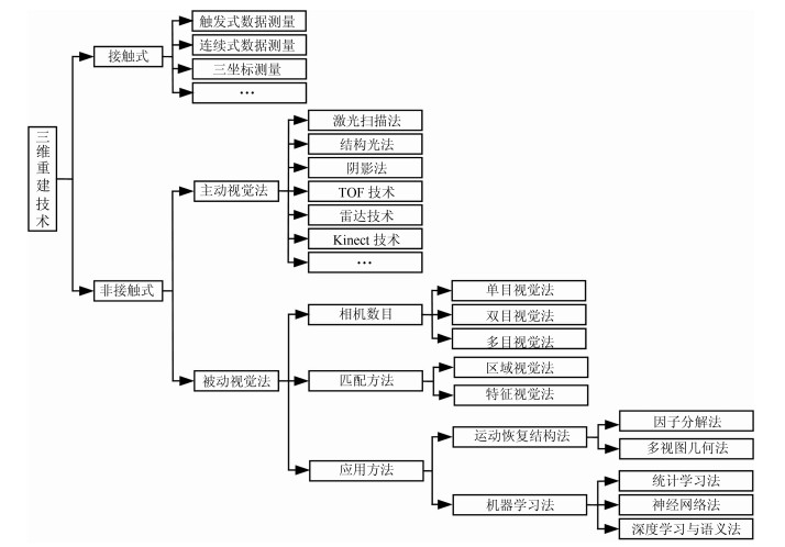
摘要: 三维重建在视觉方面具有很高的研究价值, 在机器人视觉导航、智能车环境感知系统以及虚拟现实中被广泛应用.本文对近年来国内外基于视觉的三维重建方法的研究工作进行了总结和分析, 主要介绍了基于主动视觉下的激光扫描法、结构光法、阴影法以及TOF (Time of flight)技术、雷达技术、Kinect技术和被动视觉下的单目视觉、双目视觉、多目视觉以及其他被动视觉法的三维重建技术, 并比较和分析这些方法的优点和不足.最后对三维重建的未来发展作了几点展望.Abstract: 3D reconstruction is important in vision, which can be widely used in robot vision navigation, intelligent vehicle environment perception and virtual reality. This study systematically reviews and summarizes the progress related to 3D reconstruction technology based on active vision and passive vision, i.e. laser scanning, structured light, shadow method, time of flight (TOF), radar, Kinect technology and monocular vision, binocular vision, multi-camera vision, and other passive visual methods. In addition, extensive comparisons among these methods are analyzed in detail. Finally, some perspectives on 3D reconstruction are also discussed.
-
Key words:
- 3D reconstruction /
- active vision /
- passive vision /
- key techniques
1) 本文责任编委 桑农 -

图 3 结构光三角测量原理示意图
Fig. 3 Schematic diagram of the principle of structured light triangulation
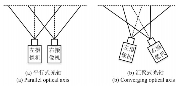
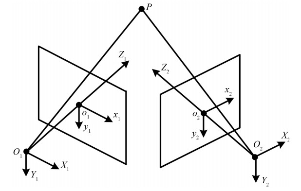
图 9 双目视觉三维重建系统组成
Fig. 9 The composition of the binocular vision 3D reconstruction system
表 1 主动视觉方法对比
Table 1 Active visual method comparison
方法 激光扫描法[28-31] 结构光法[32-42] 阴影法[43-48] TOF技术[49-53] 雷达技术[54-58] Kinect技术[59-67] 优点 1.重建结果很精确;
2.能建立形状不规则物体的三维模型.1.简单方便、无破坏性;
2.重建结果速率快、精度高、能耗低、抗干扰能力强.1.设备简单, 图像直观;
2.密度均匀, 简单低耗, 对图像的要求非常低.1.数据采集频率高;
2.垂直视场角大;
3.可以直接提取几何信息.1.视场大、扫描距离远、灵敏度高、功耗低;
2.直接获取深度信息, 不用对内部参数进行标定.1.价格便宜、轻便;
2.受光照条件的影响较小;
3.同时获取深度图像和彩色图像.缺点 1.需要采用算法来修补漏洞;
2.得到的三维点云数据量非常庞大, 而且还需要对其进行配准, 耗时较长;3.价格昂贵.1.测量速度慢;
2.不适用室外场景.1.对光照的要求较高, 需要复杂的记录装置;
2.涉及到大口径的光学部件的消像差设计、加工和调整.1.深度测量系统误差大;
2.灰度图像对比度差、分辨率低;
3.搜索空间大、效率低;
4.算法扩展性差, 空间利用率低.1.受环境的影响较大;
2.计算量较大, 实时性较差;1.深度图中含有大量的噪声;
2.对单张图像的重建效果较差. 下载: 导出CSV
表 2 单目、双目和多目视觉方法对比
Table 2 Comparison of monocular, binocular and multiocular vision methods
单目视觉[68] 双目视觉[101-110, 112] 多目视觉[111, 113-119] 优点 1.简单方便、灵活可靠、使用范围广;
2.可以实现重建过程中的摄像机自标定, 处理时间短;
3.价格便宜.1.方法成熟;
2.能够稳定地获得较好的重建效果;
3.应用广泛.1.避免双目视觉方法中难以解决的假目标、边缘模糊及误匹配等问题;
2.在多种条件下进行非接触、自动、在线的测量和检测;
3.简单方便、重建效果更好, 能够适应各种场景;缺点 1.不能够得到深度信息, 重建效果较差;
2.重建速度较慢.1.运算量大;
2.基线距离较大时重建效果降低;
3.价格较贵.1.设备结构复杂, 成本更高, 控制上难以实现;
2.实时性较低, 易受光照的影响.
下载: 导出CSV
表 3 基于视觉的三维重建技术对比与分析
Table 3 Comparison and analysis of 3D reconstruction based on vision
方法 优点 缺点 自动化程度 重建效果 实时性 应用场景 接触式方法[18] 快速直接测量物体的三维信息; 重建结果精度比较高 必须接触测量物体, 测量时物体表面容易被划伤 难以实现自动化重建 重建质量效果较好 实时 不能被广泛的应用, 只能应用到测量仪器能接触到的场景 激光扫描法[28-31] 重建的模型很精确; 重建形状不规则物体的三维模型 形成的三维点云数据量非常庞大, 不容易处理; 重建的三维模型会产生漏洞; 设备比较复杂, 价格非常昂贵 一定程度的自动化重建 重建的三维模型很好 实时 目前主要应用在工厂的生产和检测中, 无法被广泛使用 结构光法[32-42] 仅需要一幅图像就能获得物体形状; 简单方便; 无破坏性 重建速度较慢 一定程度的自动化重建 重建效果的精度比较高 实时 适用于室内场景 阴影法[43-48] 设备简单低耗; 对图像的要求非常低 对光源有一定的要求 自动化重建较低 重建效果较差, 重建过程比较复杂 实时 无法被广泛使用 TOF技术[49-53] 数据采集频率高; 垂直视场角大; 可以直接提取几何信息 深度测量系统误差大; 灰度图像对比度差、分辨率低; 搜索空间大、效率低; 算法扩展性差, 空间利用率低 一定程度的自动化重建 重建效果的精度较低 实时 能够广泛应用在人脸检测、车辆安全等方面 雷达技术[54-58] 视场大、扫描距离远、灵敏度高、功耗低; 直接获取深度信息, 不用对内部参数进行标定 受环境的影响较大; 计算量较大, 实时性较差; 价格较贵 一定程度的自动化重建 重建效果一般 实时 能够广泛应用于各行各业 Kinect技术[59-67] 价格便宜、轻便; 受光照条件的影响较小; 同时获取深度图像和彩色图像 深度图中含有大量的噪声; 对单张图像的重建效果较差 一定程度的自动化重建 重建效果较好 实时 能够被广泛应用于室内场景 明暗度法[69-72] 重建结果比较精确应用范围广泛 易受光源影响; 依赖数学运算; 鲁棒性较差 完全自动化重建 在光源比较差的情况下重建效果较差 非实时 难以应用于镜面物体以及室外场景物体的三维重建 光度立体视觉法[73-82] 避免了明暗度法存在的一些问题; 重建精度较高 易受光源影响; 鲁棒性较差 一定程度的自动化重建 重建效果较好 非实时 难以应用于镜面物体以及室外场景物体的三维重建 纹理法[83-86] 对光照和噪声都不敏感; 重建精度较高 通用性较低; 速度较快; 鲁棒性较好 完全自动化重建 重建效果的精度较高 非实时 只适用于具有规则纹理的物体 轮廓法[87-93] 重建效率非常高; 复杂度较低 对输入信息的要求很苛刻; 无法对物体表面的空洞和凹陷部分进行重建 完全自动化重建 重建效果取决于轮廓图像数量, 轮廓图像越多重建越精确 非实时 通常应用于对模型细节精度要求不是很高的三维重建中 调焦法[94-96] 对光源条件要求比较宽松; 可使用少量图像测量物体表面信息 很难实现自动重建; 需要多张图片才能进行重建 不能实现自动化重建 重建效果比较好 非实时 对纹理复杂物体的重建效果较差, 不能广泛应用 亮度法[97-100] 可全自动、无手工交互地进行高精度建模; 对光照条件要求宽松 鲁棒性较低; 灵活性较低; 复杂度较高 自动化重建 重建效果比较精细 非实时 可应用于文物数字化和人脸自动建模等领域 单目视觉法[68] 简单方便、价格便宜、灵活可靠、使用范围广; 可以实现重建过程中的摄像机自标定, 处理时间短 不能够得到深度信息, 重建速度较慢 自动化重建 重建效果较差 实时 可应用于各种场景 双目视觉法[101-110, 112] 方法成熟; 能够获得较好的重建效果 运算量大; 价格较贵; 在基线距离较大时重建效果降低 完全自动化重建 基线在一定条件下重建效果较好 实时 适用于室外场景, 应用范围广泛 多目视觉法[111, 113-119] 识别精度高, 适应性较强, 视野范围大 运算量较大; 价格昂贵, 重建时间长 完全自动化重建 基线距离较大的情况下重建效果明显降低, 而且测量精度下降, 速度受限 实时 能够适应各种场景, 在很多范围内都可以使用 区域视觉法[120-126] 计算简单; 匹配速度有所提高; 匹配精度较高; 提高了稠密匹配效率 受光线干扰较大; 对图像要求较高; 实验对象偏少 一定程度的自动化重建 重建结果较好 非实时 适用于各种领域, 例如, 视觉导航、遥感测绘 特征视觉法[154-166] 提取简单; 抗干扰能力强; 鲁棒性好; 时间和空间复杂度低 不能够对图像信息进行全面的描述 完全自动化重建 能够较精确地对物体实现三维重建 实时 应用范围较广 运动恢复结构法[127-139] 实用价值较高; 鲁棒性较强; 对图像的要求较低 计算量较大, 重建时间较长 完全自动化重建 重建效果取决于获取图像数量, 图像越多重建效果越好 实时 一般适用于大规模场景中 因子分解法[145-148] 简便灵活, 抗噪能力强, 不依赖于其他模型 精度较低, 运算时间较长 完全自动化重建 重建效果精度较低 实时 一般适用于大场景中 多视图几何法[149-163] 实用性较高; 通用性较强; 能够解决运动恢复结构法中的一些问题 计算量较大, 重建时间较长 一定程度完全自动化重建 重建效果比较好 实时 一般应用于静止的场景 统计学习法[164-173] 重建质量和效率都很高; 基本不需要人工交互 获取的信息和数据库目标不一致时, 重建结果与目标相差甚远 一定程度的自动化重建 重建效果取决于数据库的完整程度, 数据库越完备重建效果越好 非实时 适用于大场景、识别和视频检索系统 神经网络法[174-177] 精度较高, 具有很强的鲁棒性 收敛速度慢, 运算量较大 一定程度完全自动化重建 重建效果较好 实时 能够应用于各种领域, 例如计算机视觉、军事及航天等 深度学习与语义法[178-181] 计算简单, 精度较高, 不需要进行复杂的几何运算, 实时性较好 训练时间较长, 对CPU的要求较高 一定程度完全自动化重建 重建结果取决于训练的好坏 实时 适用于各种大规模场景
下载: 导出CSV
-
[1] Shen S H. Accurate multiple view 3D reconstruction using patch-based stereo for large-scale scenes. IEEE Transactions on Image Processing, 2013, 22(5): 1901-1914 doi: 10.1109/TIP.2013.2237921 [2] Qu Y F, Huang J Y, Zhang X. Rapid 3D reconstruction for image sequence acquired from UAV camera. Sensors, 2018, 18(1): 225-244 http://www.wanfangdata.com.cn/details/detail.do?_type=perio&id=sensors-18-00225 [3] Lee D Y, Park S A, Lee S J, Kim T H, Heang S, Lee J H, et al. Segmental tracheal reconstruction by 3D-printed scaffold: Pivotal role of asymmetrically porous membrane. The Laryngoscope, 2016, 126(9): E304-E309 doi: 10.1002/lary.25806 [4] Roberts L G. Machine Perception of Three-Dimensional Solids[Ph.D. dissertation], Massachusetts Institute of Technology, USA, 1963 http://www.researchgate.net/publication/37604327_Machine_perception_of_three-dimensional_solids [5] Kiyasu S, Hoshino H, Yano K, Fujimura S. Measurement of the 3-D shape of specular polyhedrons using an m-array coded light source. IEEE Transactions on Instrumentation and Measurement, 1995, 44(3): 775-778 doi: 10.1109/19.387330 [6] Snavely N, Seitz S M, Szeliski R. Photo tourism: exploring photo collections in 3D. ACM Transactions on Graphics, 2006, 25(3): 835-846 http://cn.bing.com/academic/profile?id=6d3ecda51169cc021bfe50dd9473002b&encoded=0&v=paper_preview&mkt=zh-cn [7] Pollefeys M, Nistér D, Frahm J M, Akbarzadeh A, Mordohai P, Clipp B, et al. Detailed real-time urban 3D reconstruction from video. International Journal of Computer Vision, 2008, 78(2-3): 143-167 doi: 10.1007/s11263-007-0086-4 [8] Furukawa Y, Ponce J. Carved visual hulls for image-based modeling. International Journal of Computer Vision, 2009, 81(1): 53-67 doi: 10.1007/s11263-008-0134-8 [9] Han J G, Shao L, Xu D, Shotton J. Enhanced computer vision with Microsoft Kinect sensor: a review. IEEE Transactions on Cybernetics, 2013, 43(5): 1318-1334 doi: 10.1109/TCYB.2013.2265378 [10] Ondrúška P, Kohli P, Izadi S. Mobilefusion: real-time volumetric surface reconstruction and dense tracking on mobile phones. IEEE Transactions on Visualization and Computer Graphics, 2015, 21(11): 1251-1258 doi: 10.1109/TVCG.2015.2459902 [11] 李利, 马颂德.从二维轮廓线重构三维二次曲面形状.计算机学报, 1996, 19(6): 401-408 doi: 10.3321/j.issn:0254-4164.1996.06.001Li Li, Ma Song-De. On the global quadric shape from contour. Chinese Journal of Computers, 1996, 19(6): 401-408 doi: 10.3321/j.issn:0254-4164.1996.06.001 [12] Zhong Y D, Zhang H F. Control points based semi-dense matching. In: Proceedings of the 5th Asian Conference on Computer Vision. Melbourne, Australia: ACCV, 2002. 23-25 https://www.researchgate.net/publication/237134453_Control_Points_Based_Semi-Dense_Matching [13] 雷成, 胡占义, 吴福朝, Tsui H T.一种新的基于Kruppa方程的摄像机自标定方法.计算机学报, 2003, 26(5): 587-597 doi: 10.3321/j.issn:0254-4164.2003.05.010Lei Cheng, Hu Zhan-Yi, Wu Fu-Chao, Tsui H T. A novel camera self-calibration technique based on the Kruppa equations. Chinese Journal of Computers, 2003, 26(5): 587-597 doi: 10.3321/j.issn:0254-4164.2003.05.010 [14] 雷成, 吴福朝, 胡占义.一种新的基于主动视觉系统的摄像机自标定方法.计算机学报, 2000, 23(11): 1130-1139 doi: 10.3321/j.issn:0254-4164.2000.11.002Lei Cheng, Wu Fu-Chao, Hu Zhan-Yi. A new camera self-calibration method based on active vision system. Chinese Journal of Computer, 2000, 23(11): 1130-1139 doi: 10.3321/j.issn:0254-4164.2000.11.002 [15] 张涛.基于单目视觉的三维重建[硕士学位论文], 西安电子科技大学, 中国, 2014 http://cdmd.cnki.com.cn/Article/CDMD-10701-1014325012.htmZhang Tao. 3D Reconstruction Based Monocular Vision[Master thesis], Xidian University, China, 2014 http://cdmd.cnki.com.cn/Article/CDMD-10701-1014325012.htm [16] Ebrahimnezhad H, Ghassemian H. Robust motion from space curves and 3D reconstruction from multiviews using perpendicular double stereo rigs. Image and Vision Computing, 2008, 26(10): 1397-1420 doi: 10.1016/j.imavis.2008.01.002 [17] Hartley R, Zisserman A. Multiple View Geometry in Computer Vision. New York: Cambridge University Press, 2003 [18] Várady T, Martin R R, Cox J. Reverse engineering of geometric models—an introduction. Computer-Aided Design, 1997, 29(4): 255-268 doi: 10.1016/S0010-4485(96)00054-1 [19] Isgro F, Odone F, Verri A. An open system for 3D data acquisition from multiple sensor. In: Proceedings of the 7th International Workshop on Computer Architecture for Machine Perception. Palermo, Italy: IEEE, 2005. 52-57 https://www.researchgate.net/publication/221210593_An_Open_System_for_3D_Data_Acquisition_from_Multiple_Sensor?ev=auth_pub [20] Williams C G, Edwards M A, Colley A L, Macpherson J V, Unwin P R. Scanning micropipet contact method for high-resolution imaging of electrode surface redox activity. Analytical Chemistry, 2009, 81(7): 2486-2495 doi: 10.1021/ac802114r [21] Kraus K, Pfeifer N. Determination of terrain models in wooded areas with airborne laser scanner data. ISPRS Journal of Photogrammetry and Remote Sensing, 1998, 53(4): 193-203 doi: 10.1016/S0924-2716(98)00009-4 [22] Göbel W, Kampa B M, Helmchen F. Imaging cellular network dynamics in three dimensions using fast 3D laser scanning. Nature Methods, 2007, 4(1): 73-79 doi: 10.1038/nmeth989 [23] Rocchini C, Cignoni P, Montani C, Pingi P, Scopigno R. A low cost 3D scanner based on structured light. Computer Graphics Forum, 2001, 20(3): 299-308 doi: 10.1111/1467-8659.00522 [24] Al-Najdawi N, Bez H E, Singhai J, Edirisinghe E A. A survey of cast shadow detection algorithms. Pattern Recognition Letters, 2012, 33(6): 752-764 http://www.wanfangdata.com.cn/details/detail.do?_type=perio&id=0edff8a864c6e0b39fa06480e789be36 [25] Park J, Kim H, Tai Y W, Brown M S, Kweon I. High quality depth map upsampling for 3d-tof cameras. In: Proceedings of the 2011 International Conference on Computer Vision. Barcelona, Spain: IEEE, 2011. 1623-1630 https://www.researchgate.net/publication/221110931_High_Quality_Depth_Map_Upsampling_for_3D-TOF_Cameras [26] Schwarz B. LIDAR: mapping the world in 3D. Nature Photonics, 2010, 4(7): 429-430 doi: 10.1038/nphoton.2010.148 [27] Khoshelham K, Elberink S O. Accuracy and resolution of kinect depth data for indoor mapping applications. Sensors, 2012, 12(2): 1437-1454 doi: 10.3390/s120201437 [28] 杨耀权, 施仁, 于希宁, 高镗年.激光扫描三角法大型曲面测量中影响参数分析.西安交通大学学报, 1999, 33(7): 15-18 doi: 10.3321/j.issn:0253-987X.1999.07.005Yang Yao-Quan, Shi Ren, Yu Xi-Ning, Gao Tang-Nian. Laser scanning triangulation for large profile measurement. Journal of Xi'an Jiaotong University, 1999, 33(7): 15-18 doi: 10.3321/j.issn:0253-987X.1999.07.005 [29] Boehler W, Vicent M B, Marbs A. Investigating laser scanner accuracy. The International Archives of Photogrammetry, Remote Sensing and Spatial Information Sciences, 2003, 34(5): 696-701 https://www.researchgate.net/publication/246536800_Investigating_laser_scanner_accuracy [30] Reshetyuk Y. Investigation and Calibration of Pulsed Time-of-Flight Terrestrial Laser Scanners[Master dissertation], Royal Institute of Technology, Switzerland, 2006. 14-17 https://www.researchgate.net/publication/239563997_Investigation_and_calibration_of_pulsed_time-of-flight_terrestrial_laser_scanners [31] Voisin S, Foufou S, Truchetet F, Page D L, Abidi M A. Study of ambient light influence for three-dimensional scanners based on structured light. Optical Engineering, 2007, 46(3): Article No. 030502 http://www.wanfangdata.com.cn/details/detail.do?_type=perio&id=dd6f1c5d53c51efe4c6ad10b4ed19e5e [32] Scharstein D, Szeliski R. High-accuracy stereo depth maps using structured light. In: Proceedings of the 2003 IEEE Computer Society Conference on Computer Vision and Pattern Recognition. Madison, WI, USA: IEEE, 2003. I-195-I-202 https://www.researchgate.net/publication/4022931_High-accuracy_stereo_depth_maps_using_structured_light [33] Chen F, Brown G M, Song M M. Overview of 3-D shape measurement using optical methods. Optical Engineering, 2000, 39(1): 10-22 doi: 10.1117/1.602438 [34] Pollefeys M, Van Gool L. Stratified self-calibration with the modulus constraint. IEEE Transactions on Pattern Analysis and Machine Intelligence, 1999, 21(8): 707-724 doi: 10.1109/34.784285 [35] O'Toole M, Mather J, Kutulakos K N. 3D shape and indirect appearance by structured light transport. IEEE Transactions on Pattern Analysis and Machine Intelligence, 2016, 38(7): 1298-1312 doi: 10.1109/TPAMI.2016.2545662 [36] Song Z, Chung R. Determining both surface position and orientation in structured-light-based sensing. IEEE Transactions on Pattern Analysis and Machine Intelligence, 2010, 32(10): 1770-1780 doi: 10.1109/TPAMI.2009.192 [37] Kowarschik R, Kuehmstedt P, Gerber J, Schreiber W, Notni G. Adaptive optical 3-D-measurement with structured light. Optical Engineering, 2000, 39(1): 150-158 doi: 10.1117/1.602346 [38] Shakhnarovich G, Viola P A, Moghaddam B. A unified learning framework for real time face detection and classification. In: Proceedings of the 5th IEEE International Conference on Automatic Face Gesture Recognition. Washington, USA: IEEE, 2002. 14-21 https://www.researchgate.net/publication/262436645_A_unified_learning_framework_for_real_time_face_detection_and_classification [39] Salvi J, Pagès J, Batlle J. Pattern codification strategies in structured light systems. Pattern Recognition, 2004, 37(4): 827-849 doi: 10.1016/j.patcog.2003.10.002 [40] 张广军, 李鑫, 魏振忠.结构光三维双视觉检测方法研究.仪器仪表学报, 2002, 23(6): 604-607, 624 doi: 10.3321/j.issn:0254-3087.2002.06.014Zhang Guang-Jun, Li Xin, Wei Zhen-Zhong. A method of 3D double-vision inspection based on structured light. Chinese Journal of Scientific Instrument, 2002, 23(6): 604-607, 624 doi: 10.3321/j.issn:0254-3087.2002.06.014 [41] 王宝光, 贺忠海, 陈林才, 倪勇.结构光传感器模型及特性分析.光学学报, 2002, 22(4): 481-484 doi: 10.3321/j.issn:0253-2239.2002.04.022Wang Bao-Guang, He Zhong-Hai, Chen Lin-Cai, Ni Yong. Model and performance analysis of structured light sensor. Acta Optica Sinica, 2002, 22(4): 481-484 doi: 10.3321/j.issn:0253-2239.2002.04.022 [42] 罗先波, 钟约先, 李仁举.三维扫描系统中的数据配准技术.清华大学学报(自然科学版), 2004, 44(8): 1104-1106 doi: 10.3321/j.issn:1000-0054.2004.08.028Luo Xian-Bo, Zhong Yue-Xian, Li Ren-Ju. Data registration in 3-D scanning systems. Journal of Tsinghua University (Science and Technology), 2004, 44(8): 1104-1106 doi: 10.3321/j.issn:1000-0054.2004.08.028 [43] Savarese S, Andreetto M, Rushmeier H, Bernardini F, Perona P. 3D reconstruction by shadow carving: theory and practical evaluation. International Journal of Computer Vision, 2007, 71(3): 305-336 doi: 10.1007/s11263-006-8323-9 [44] Wang Y X, Cheng H D, Shan J. Detecting shadows of moving vehicles based on HMM. In: Proceedings of the 19th International Conference on Pattern Recognition. Tampa, FL, USA: IEEE, 2008. 1-4 [45] Rüfenacht D, Fredembach C, Süsstrunk S. Automatic and accurate shadow detection using near-infrared information. IEEE Transactions on Pattern Analysis and Machine Intelligence, 2014, 36(8): 1672-1678 doi: 10.1109/TPAMI.2013.229 [46] Daum M, Dudek G. On 3-D surface reconstruction using shape from shadows. In: Proceedings of the 1998 IEEE Computer Society Conference on Computer Vision and Pattern Recognition. Santa Barbara, CA, USA: IEEE, 1998. 461-468 http://www.researchgate.net/publication/3758700_On_3-D_surface_reconstruction_using_shape_from_shadows [47] Woo A, Poulin P, Fournier A. A survey of shadow algorithms. IEEE Computer Graphics and Applications, 1990, 10(6): 13-32 http://d.old.wanfangdata.com.cn/Periodical/xxykz201502016 [48] Hasenfratz J M, Lapierre M, Holzschuch N, Sillion F, Gravir/Imag-Inria A. A survey of real-time soft shadows algorithms. Computer Graphics Forum, 2003, 22(4): 753-774 doi: 10.1111/j.1467-8659.2003.00722.x [49] May S, Droeschel D, Holz D, Wiesen C. 3D pose estimation and mapping with time-of-flight cameras. In: Proceedings of IEEE/RSJ International Conference on Intelligent Robots and Systems. Nice, France: IEEE, 2008. 120-125 https://www.researchgate.net/publication/228662715_3D_pose_estimation_and_mapping_with_time-of-flight_cameras [50] Hegde G P M, Ye C. Extraction of planar features from swissranger sr-3000 range images by a clustering method using normalized cuts. In: Proceedings of the 2009 IEEE/RSJ International Conference on Intelligent Robots and Systems. St. Louis, MO, USA: IEEE, 2009. 4034-4039 https://www.researchgate.net/publication/224090431_Extraction_of_Planar_Features_from_Swissranger_SR-3000_Range_Images_by_a_Clustering_Method_Using_Normalized_Cuts [51] Pathak K, Vaskevicius N, Poppinga J, Pfingsthorn M, Schwertfeger S, Birk A. Fast 3D mapping by matching planes extracted from range sensor point-clouds. In: Proceedings of the 2009 IEEE/RSJ International Conference on Intelligent Robots and Systems. St. Louis, MO, USA: IEEE, 2009. 1150-1155 http://www.researchgate.net/publication/224090528_Fast_3D_mapping_by_matching_planes_extracted_from_range_sensor_point-clouds?ev=auth_pub [52] Stipes J A, Cole J G P, Humphreys J. 4D scan registration with the SR-3000 LIDAR. In: Proceedings of the 2008 IEEE International Conference on Robotics and Automation. Pasadena, CA, USA: IEEE, 2008. 2988-2993 http://www.researchgate.net/publication/224318679_4d_scan_registration_with_the_sr-3000_lidar [53] May S, Droeschel D, Fuchs S, Holz D, Nüchter A. Robust 3D-mapping with time-of-flight cameras. In: Proceedings of the 2009 IEEE/RSJ International Conference on Intelligent Robots and Systems. St. Louis, MO, USA: IEEE, 2009. 1673-1678 https://www.researchgate.net/publication/46160281_3D_mapping_with_time-of-flight_cameras [54] Streller D, Dietmayer K. Object tracking and classification using a multiple hypothesis approach. In: Proceedings of the 2004 IEEE Intelligent Vehicles Symposium. Parma, Italy: IEEE, 2004. 808-812 https://www.researchgate.net/publication/4092472_Object_tracking_and_classification_using_a_multiple_hypothesis_approach [55] Schwalbe E, Maas H G, Seidel F. 3D building model generation from airborne laser scanner data using 2D GIS data and orthogonal point cloud projections. In: Proceedings of ISPRS WG Ⅲ/3, Ⅲ/4, V/3 Workshop "Laser Scanning 2005". Enschede, the Netherlands: IEEE, 2005. 12-14 https://www.researchgate.net/publication/228681223_3D_building_model_generation_from_airborne_laser_scanner_data_using_2D_GIS_data_and_orthogonal_point_cloud_projections [56] Weiss T, Schiele B, Dietmayer K. Robust driving path detection in urban and highway scenarios using a laser scanner and online occupancy grids. In: Proceedings of the 2007 IEEE Intelligent Vehicles Symposium. Istanbul, Turkey: IEEE, 2007. 184-189 https://www.researchgate.net/publication/4268869_Robust_Driving_Path_Detection_in_Urban_and_Highway_Scenarios_Using_a_Laser_Scanner_and_Online_Occupancy_Grids [57] 胡明.基于点云数据的重建算法研究[硕士学位论文], 华南理工大学, 中国, 2010 http://cdmd.cnki.com.cn/Article/CDMD-10561-1011044410.htmHu Ming. Algorithm Reconstruction Based on Cloud Data[Master thesis], South China University of Technology, China, 2010 http://cdmd.cnki.com.cn/Article/CDMD-10561-1011044410.htm [58] 魏征.车载LiDAR点云中建筑物的自动识别与立面几何重建[博士学位论文], 武汉大学, 中国, 2012 http://cdmd.cnki.com.cn/Article/CDMD-10486-1013151916.htmWei Zheng. Automated Extraction of Buildings and Facades Reconstructon from Mobile LiDAR Point Clouds[Ph.D. dissertation], Wuhan University, China, 2012 http://cdmd.cnki.com.cn/Article/CDMD-10486-1013151916.htm [59] Zhang Z Y. Microsoft kinect sensor and its effect. IEEE Multimedia, 2012, 19(2): 4-10 doi: 10.1109/MMUL.2012.24 [60] Zhang Z. A flexible new technique for camera calibration. IEEE Transactions on Pattern Analysis and Machine Intelligence, 2000, 22(11): 1330-1334 doi: 10.1109/34.888718 [61] Smisek J, Jancosek M, Pajdla T. 3D with Kinect. In: Proceedings of the 2011 IEEE International Conference on Computer Vision. Barcelona, Spain: IEEE, 2011. 1154-1160 http://www.researchgate.net/publication/221429935_3D_with_Kinect [62] Zollhöfer M, Nießner M, Izadi S, Rehmann C, Zach C, Fisher M, et al. Real-time non-rigid reconstruction using an RGB-D camera. ACM Transactions on Graphics, 2014, 33(4): Article No. 156 http://d.old.wanfangdata.com.cn/NSTLQK/NSTL_QKJJ0234048647/ [63] Henry P, Krainin M, Herbst E, Ren X F, Fox D. RGB-D mapping: using depth cameras for dense 3D modeling of indoor environments. Experimental Robotics: the 12th International Symposium on Experimental Robotics. Heidelberg, Germany: Springer, 2014. 477-491 doi: 10.1007%2F978-3-642-28572-1_33 [64] Henry P, Krainin M, Herbst E, Ren X F, Fox D. RGB-D mapping: using Kinect-style depth cameras for dense 3D modeling of indoor environments. The International Journal of Robotics Research, 2012, 31(5): 647-663 doi: 10.1177/0278364911434148 [65] Newcombe R A, Izadi S, Hilliges O, Molyneaux D, Kim D, Davison A J, et al. KinectFusion: real-time dense surface mapping and tracking. In: Proceedings of the 10th IEEE International Symposium on Mixed and Augmented Reality. Basel, Switzerland: IEEE, 2011. 127-136 http://www.researchgate.net/publication/224266200_KinectFusion_Real-time_dense_surface_mapping_and_tracking [66] Izadi S, Kim D, Hilliges O, Molyneaux D, Newcombe R, Kohli P, et al. KinectFusion: real-time 3D reconstruction and interaction using a moving depth camera. In: Proceedings of the 24th Annual ACM Symposium on User Interface Software and Technology. Santa Barbara, California, USA: ACM, 2011. 559-568 https://www.researchgate.net/publication/220877151_KinectFusion_Real-time_3D_reconstruction_and_interaction_using_a_moving_depth_camera [67] 吴侗.基于点云多平面检测的三维重建关键技术研究[硕士学位论文], 南昌航空大学, 中国, 2013 http://cdmd.cnki.com.cn/Article/CDMD-10406-1014006472.htmWu Tong. Research on Key Technologies of 3D Reconstruction Based on Multi-plane Detection in Point Clouds[Master thesis], Nanchang Hangkong University, China, 2013 http://cdmd.cnki.com.cn/Article/CDMD-10406-1014006472.htm [68] 佟帅, 徐晓刚, 易成涛, 邵承永.基于视觉的三维重建技术综述.计算机应用研究, 2011, 28(7): 2411-2417 doi: 10.3969/j.issn.1001-3695.2011.07.003Tong Shuai, Xu Xiao-Gang, Yi Cheng-Tao, Shao Cheng-Yong. Overview on vision-based 3D reconstruction. Application Research of Computers, 2011, 28(7): 2411-2417 doi: 10.3969/j.issn.1001-3695.2011.07.003 [69] Horn B K P. Shape from Shading: A Method for Obtaining the Shape of A Smooth Opaque Object from One View[Ph.D. dissertation], Massachusetts Institute of Technology, USA, 1970 http://www.researchgate.net/publication/37602086_Shape_from_shading_a_method_for_obtaining_the_shape_of_a_smooth_opaque_object_from_one_view [70] Penna M A. A shape from shading analysis for a single perspective image of a polyhedron. IEEE Transactions on Pattern Analysis and Machine Intelligence, 1989, 11(6): 545-554 doi: 10.1109/34.24790 [71] Bakshi S, Yang Y H. Shape from shading for non-Lambertian surfaces. In: Proceedings of the 1st International Conference on Image Processing. Austin, USA: IEEE, 1994. 130-134 https://www.researchgate.net/publication/2822887_Shape_From_Shading_for_Non-Lambertian_Surfaces [72] Vogel O, Breuß M, Weickert J. Perspective shape from shading with non-Lambertian reflectance. Pattern Recognition. Heidelberg, Germany: Springer, 2008. 517-526 doi: 10.1007/978-3-540-69321-5_52.pdf [73] Woodham R J. Photometric method for determining surface orientation from multiple images. Optical Engineering, 1980, 19(1): Article No. 191139 http://www.wanfangdata.com.cn/details/detail.do?_type=perio&id=CC024631993 [74] Noakes L, Kozera R. Nonlinearities and noise reduction in 3-source photometric stereo. Journal of Mathematical Imaging and Vision, 2003, 18(2): 119-127 doi: 10.1023/A:1022104332058 [75] Horovitz I, Kiryati N. Depth from gradient fields and control points: bias correction in photometric stereo. Image and Vision Computing, 2004, 22(9): 681-694 doi: 10.1016/j.imavis.2004.01.005 [76] Tang K L, Tang C K, Wong T T. Dense photometric stereo using tensorial belief propagation. In: Proceedings of the 2005 IEEE Computer Society Conference on Computer Vision and Pattern Recognition. San Diego, USA: IEEE, 2005. 132-139 http://www.researchgate.net/publication/4156302_Dense_photometric_stereo_using_tensorial_belief_propagation [77] Xie H, Pierce L E, Ulaby F T. SAR speckle reduction using wavelet denoising and Markov random field modeling. IEEE Transactions on Geoscience and Remote Sensing, 2002, 40(10): 2196-2212 doi: 10.1109/TGRS.2002.802473 [78] Sun J A, Smith M, Smith L, Midha S, Bamber J. Object surface recovery using a multi-light photometric stereo technique for non-Lambertian surfaces subject to shadows and specularities. Image and Vision Computing, 2007, 25(7): 1050-1057 doi: 10.1016/j.imavis.2006.04.025 [79] Vlasic D, Peers P, Baran I, Debevec P, Popović J, Rusinkiewicz S, et al. Dynamic shape capture using multi-view photometric stereo. ACM Transactions on Graphics, 2009, 28(5): Article No. 174 http://d.old.wanfangdata.com.cn/NSTLQK/NSTL_QKJJ0216027840/ [80] Shi B X, Matsushita Y, Wei Y C, Xu C, Tan P. Self-calibrating photometric stereo. In: Proceedings of the 2010 IEEE Computer Society Conference on Computer Vision and Pattern Recognition. San Francisco, USA: IEEE, 2010. 1118-1125 http://www.researchgate.net/publication/221363790_Self-calibrating_photometric_stereo [81] Morris N J W, Kutulakos K N. Dynamic refraction stereo. IEEE Transactions on Pattern Analysis and Machine Intelligence, 2011, 33(8): 1518-1531 doi: 10.1109/TPAMI.2011.24 [82] Higo T, Matsushita Y, Ikeuchi K. Consensus photometric stereo. In: Proceedings of the 2010 IEEE Computer Society Conference on Computer Vision and Pattern Recognition. San Francisco, USA: IEEE, 2010. 1157-1164 http://www.researchgate.net/publication/221363482_Consensus_photometric_stereo [83] Brown L G, Shvaytser H. Surface orientation from projective foreshortening of isotropic texture autocorrelation. In: Proceedings of the 1988 Computer Society Conference on Computer Vision and Pattern Recognition. Ann Arbor, USA: IEEE, 1988. 510-514 http://www.researchgate.net/publication/3497773_Surface_orientation_from_projective_foreshortening_of_isotropictexture_autocorrelation [84] Clerc M, Mallat S. The texture gradient equation for recovering shape from texture. IEEE Transactions on Pattern Analysis and Machine Intelligence, 2002, 24(4): 536-549 doi: 10.1109/34.993560 [85] Witkin A P. Recovering surface shape and orientation from texture. Artificial Intelligence, 1981, 17(1-3): 17-45 doi: 10.1016/0004-3702(81)90019-9 [86] Warren P A, Mamassian P. Recovery of surface pose from texture orientation statistics under perspective projection. Biological Cybernetics, 2010, 103(3): 199-212 doi: 10.1007/s00422-010-0389-3 [87] Martin W N, Aggarwal J K. Volumetric descriptions of objects from multiple views. IEEE Transactions on Pattern Analysis and Machine Intelligence, 1983, PAMI-5(2): 150-158 doi: 10.1109/TPAMI.1983.4767367 [88] Laurentini A. The visual hull concept for silhouette-based image understanding. IEEE Transactions on Pattern Analysis and Machine Intelligence, 1994, 16(2): 150-162 doi: 10.1109/34.273735 [89] Bongiovanni G, Guerra C, Levialdi S. Computing the Hough transform on a pyramid architecture. Machine Vision and Applications, 1990, 3(2): 117-123 doi: 10.1007/BF01212195 [90] Darell T, Wohn K. Depth from focus using a pyramid architecture. Pattern Recognition Letters, 1990, 11(12): 787-796 doi: 10.1016/0167-8655(90)90032-W [91] Kavianpour A, Bagherzadeh N. Finding circular shapes in an image on a pyramid architecture. Pattern Recognition Letters, 1992, 13(12): 843-848 doi: 10.1016/0167-8655(92)90083-C [92] Forbes K, Nicolls F, De Jager G, Voigt A. Shape-from-silhouette with two mirrors and an uncalibrated camera. In: Proceedings of the 9th European Conference on Computer Vision. Graz, Austria: Springer, 2006. 165-178 doi: 10.1007/11744047_13.pdf [93] Lehtinen J, Aila T, Chen J W, Laine S, Durand F. Temporal light field reconstruction for rendering distribution effects. ACM Transactions on Graphics, 2011, 30(4): Article No. 55 http://cn.bing.com/academic/profile?id=f48b75e3f65df6c92db0ec3ba3f22ce9&encoded=0&v=paper_preview&mkt=zh-cn [94] Nayar S K, Nakagawa Y. Shape from focus. IEEE Transactions on Pattern Analysis and Machine Intelligence, 1994, 16(8): 824-831 doi: 10.1109/34.308479 [95] Hasinoff S W, Kutulakos K N. Confocal stereo. International Journal of Computer Vision, 2009, 81(1): 82-104 doi: 10.1007/s11263-008-0164-2 [96] Pradeep K S, Rajagopalan A N. Improving shape from focus using defocus cue. IEEE Transactions on Image Processing, 2007, 16(7): 1920-1925 doi: 10.1109/TIP.2007.899188 [97] Slabaugh G G, Culbertson W B, Malzbender T, Stevens M R, Schafer R W. Methods for volumetric reconstruction of visual scenes. International Journal of Computer Vision, 2004, 57(3): 179-199 doi: 10.1023/B:VISI.0000013093.45070.3b [98] de Vries S C, Kappers A M L, Koenderink J J. Shape from stereo: a systematic approach using quadratic surfaces. Perception & Psychophysics, 1993, 53(1): 71-80 http://cn.bing.com/academic/profile?id=23f384adcd3565fda27091b0a353d075&encoded=0&v=paper_preview&mkt=zh-cn [99] Seitz S M, Dyer C R. Photorealistic scene reconstruction by voxel coloring. International Journal of Computer Vision, 1999, 35(2): 151-173 doi: 10.1023/A:1008176507526 [100] Kutulakos K N, Seitz S M. A theory of shape by space carving. International Journal of Computer Vision, 2000, 38(3): 199-218 doi: 10.1023/A:1008191222954 [101] Li D W, Xu L H, Tang X S, Sun S Y, Cai X, Zhang P. 3D imaging of greenhouse plants with an inexpensive binocular stereo vision system. Remote Sensing, 2017, 9(5): Article No. 508 doi: 10.3390/rs9050508 [102] Helveston E M, Boudreault G. Binocular vision and ocular motility: theory and management of strabismus. American Journal of Ophthalmology, 1986, 101(1): 135 http://d.old.wanfangdata.com.cn/OAPaper/oai_pubmedcentral.nih.gov_2590061 [103] Qi F, Zhao D B, Gao W. Reduced reference stereoscopic image quality assessment based on binocular perceptual information. IEEE Transactions on Multimedia, 2015, 17(12): 2338-2344 doi: 10.1109/TMM.2015.2493781 [104] Sizintsev M, Wildes R P. Spacetime stereo and 3D flow via binocular spatiotemporal orientation analysis. IEEE Transactions on Pattern Analysis and Machine Intelligence, 2014, 36(11): 2241-2254 doi: 10.1109/TPAMI.2014.2321373 [105] Marr D, Poggio T. A computational theory of human stereo vision. Proceedings of the Royal Society B: Biological Sciences, 1979, 204(1156): 301-328 http://www.wanfangdata.com.cn/details/detail.do?_type=perio&id=CC026931228 [106] Zou X J, Zou H X, Lu J. Virtual manipulator-based binocular stereo vision positioning system and errors modelling. Machine Vision and Applications, 2012, 23(1): 43-63 http://d.old.wanfangdata.com.cn/NSTLQK/NSTL_QKJJ0225968290/ [107] 李占贤, 许哲.双目视觉的成像模型分析.机械工程与自动化, 2014, (4): 191-192 doi: 10.3969/j.issn.1672-6413.2014.04.081Li Zhan-Xian, Xu Zhe. Analysis of imaging model of binocular vision. Mechanical Engineering & Automation, 2014, (4): 191-192 doi: 10.3969/j.issn.1672-6413.2014.04.081 [108] 张文明, 刘彬, 李海滨.基于双目视觉的三维重建中特征点提取及匹配算法的研究.光学技术, 2008, 34(2): 181-185 doi: 10.3321/j.issn:1002-1582.2008.02.039Zhang Wen-Ming, Liu Bin, Li Hai-Bin. Characteristic point extracts and the match algorithm based on the binocular vision in three dimensional reconstruction. Optical Technique, 2008, 34(2): 181-185 doi: 10.3321/j.issn:1002-1582.2008.02.039 [109] Bruno F, Bianco G, Muzzupappa M, Barone S, Razionale A V. Experimentation of structured light and stereo vision for underwater 3D reconstruction. ISPRS Journal of Photogrammetry and Remote Sensing, 2011, 66(4): 508-518 doi: 10.1016/j.isprsjprs.2011.02.009 [110] Fusiello A, Trucco E, Verri A. A compact algorithm for rectification of stereo pairs. Machine Vision and Applications, 2000, 12(1): 16-22 doi: 10.1007/s001380050120 [111] Baillard C, Zisserman A. A plane-sweep strategy for the 3D reconstruction of buildings from multiple images. In: Proceedings of the 2000 International Archives of Photogrammetry and Remote Sensing. Amsterdam, Netherlands: ISPRS, 2000. 56-62 https://www.researchgate.net/publication/2813005_A_Plane-Sweep_Strategy_For_The_3D_Reconstruction_Of_Buildings_From_Multiple_Images [112] Hirschmuller H, Scharstein D. Evaluation of stereo matching costs on images with radiometric differences. IEEE Transactions on Pattern Analysis and Machine Intelligence, 2009, 31(9): 1582-1599 doi: 10.1109/TPAMI.2008.221 [113] Zhang T, Liu J H, Liu S L, Tang C T, Jin P. A 3D reconstruction method for pipeline inspection based on multi-vision. Measurement, 2017, 98: 35-48 doi: 10.1016/j.measurement.2016.11.004 [114] Saito K, Miyoshi T, Yoshikawa H. Noncontact 3-D digitizing and machining system for free-form surfaces. CIRP Annals, 1991, 40(1): 483-486 doi: 10.1016/S0007-8506(07)62035-6 [115] 陈明舟.主动光栅投影双目视觉传感器的研究[硕士学位论文], 天津大学, 中国, 2002 http://www.wanfangdata.com.cn/details/detail.do?_type=degree&id=Y456511Chen Ming-Zhou. Research on Active Grating Projection Stereo Vision Sensor[Master thesis], Tianjin University, China, 2002 http://www.wanfangdata.com.cn/details/detail.do?_type=degree&id=Y456511 [116] 王磊.三维重构技术的研究与应用[硕士学位论文], 清华大学, 中国, 2002Wang Lei. The Research and Application of 3D Reconstruction Technology[Master thesis], Tsinghua University, China, 2002 [117] Hernández C, Vogiatzis G, Cipolla R. Overcoming shadows in 3-source photometric stereo. IEEE Transactions on Pattern Analysis and Machine Intelligence, 2011, 33(2): 419-426 doi: 10.1109/TPAMI.2010.181 [118] Park H, Lee H, Sull S. Efficient viewer-centric depth adjustment based on virtual fronto-parallel planar projection in stereo 3D images. IEEE Transactions on Multimedia, 2014, 16(2): 326-336 doi: 10.1109/TMM.2013.2286567 [119] Bai X, Rao C, Wang X G. Shape vocabulary: a robust and efficient shape representation for shape matching. IEEE Transactions on Image Processing, 2014, 23(9): 3935-3949 doi: 10.1109/TIP.2014.2336542 [120] Goshtasby A, Stockman G C, Page C V. A region-based approach to digital image registration with subpixel accuracy. IEEE Transactions on Geoscience and Remote Sensing, 1986, GE-24 (3): 390-399 doi: 10.1109/TGRS.1986.289597 [121] Flusser J, Suk T. A moment-based approach to registration of images with affine geometric distortion. IEEE Transactions on Geoscience and Remote Sensing, 1994, 32(2): 382-387 doi: 10.1109/36.295052 [122] Alhichri H S, Kamel M. Virtual circles: a new set of features for fast image registration. Pattern Recognition Letters, 2003, 24(9-10): 1181-1190 doi: 10.1016/S0167-8655(02)00300-8 [123] Schmid C, Mohr R. Local grayvalue invariants for image retrieval. IEEE Transactions on Pattern Analysis and Machine Intelligence, 1997, 19(5): 530-535 doi: 10.1109/34.589215 [124] Matas J, Chum O, Urban M, Pajdla T. Robust wide-baseline stereo from maximally stable extremal regions. Image and Vision Computing, 2004, 22(10): 761-767 doi: 10.1016/j.imavis.2004.02.006 [125] Tuytelaars T, Van Gool L. Matching widely separated views based on affine invariant regions. International Journal of Computer Vision, 2004, 59(1): 61-85 doi: 10.1023/B:VISI.0000020671.28016.e8 [126] Kadir T, Zisserman A, Brady M. An affine invariant salient region detector. In: Proceedings of the 8th European Conference on Computer Vision. Prague, Czech Republic: Springer, 2004. 228-241 http://www.researchgate.net/publication/2909469_An_Ane_Invariant_Salient_Region_Detector [127] Harris C, Stephens M. A combined corner and edge detector. In: Proceedings of the 4th Alvey Vision Conference. 1988. 1475-151 https://www.researchgate.net/publication/215458771_A_Combined_Corner_and_Edge_Detector [128] Morevec H P. Towards automatic visual obstacle avoidance. In: Proceedings of the 5th International Joint Conference on Artificial Intelligence. Cambridge, USA: ACM, 1977. 584 https://www.researchgate.net/publication/220814569_Towards_Automatic_Visual_Obstacle_Avoidance [129] Schmid C, Mohr R, Bauckhage C. Evaluation of interest point detectors. International Journal of Computer Vision, 2000, 37(2): 151-172 doi: 10.1023/A:1008199403446 [130] Van de Weijer J, Gevers T, Bagdanov A D. Boosting color saliency in image feature detection. IEEE Transactions on Pattern Analysis and Machine Intelligence, 2006, 28(1): 150-156 doi: 10.1109/TPAMI.2006.3 [131] Mikolajczyk K, Schmid C. Scale & affine invariant interest point detectors. International Journal of Computer Vision, 2004, 60(1): 63-86 https://www.researchgate.net/publication/215721498_Scale_Affine_Invariant_Interest_Point_Detectors [132] Smith S M, Brady J M. SUSAN — a new approach to low level image processing. International Journal of Computer Vision, 1997, 23(1): 45-78 doi: 10.1023/A:1007963824710 [133] Lindeberg T, Gårding J. Shape-adapted smoothing in estimation of 3-D shape cues from affine deformations of local 2-D brightness structure. Image and Vision Computing, 1997, 15(6): 415-434 doi: 10.1016/S0262-8856(97)01144-X [134] Lindeberg T. Feature detection with automatic scale selection. International Journal of Computer Vision, 1998, 30(2): 79-116 doi: 10.1023/A:1008045108935 [135] Baumberg A. Reliable feature matching across widely separated views. In: Proceedings of the 2000 IEEE Conference on Computer Vision and Pattern Recognition. Hilton Head Island, USA: IEEE, 2000. 774-781 [136] Lowe D G. Object recognition from local scale-invariant features. In: Proceedings of the 7th IEEE International Conference on Computer Vision. Kerkyra, Greece: IEEE, 1999. 1150-1157 [137] Ke Y, Sukthankar R. PCA-SIFT: a more distinctive representation for local image descriptors. In: Proceedings of the 2004 IEEE Computer Society Conference on Computer Vision and Pattern Recognition. Washington D.C., USA: IEEE, 2004. Ⅱ-506-Ⅱ-513 http://www.researchgate.net/publication/2926479_PCA-SIFT_A_More_Distinctive_Representation_for_Local_Image_Descriptors [138] Bay H, Tuytelaars T, Van Gool L. SURF: speeded up robust features. In: Proceedings of the 9th European Conference on Computer Vision. Graz, Austria: Springer, 2006. 404-417 [139] 葛盼盼, 陈强, 顾一禾.基于Harris角点和SURF特征的遥感图像匹配算法.计算机应用研究, 2014, 31(7): 2205-2208 doi: 10.3969/j.issn.1001-3695.2014.07.069Ge Pan-Pan, Chen Qiang, Gu Yi-He. Algorithm of remote sensing image matching based on Harris corner and SURF feature. Application Research of Computers, 2014, 31(7): 2205-2208 doi: 10.3969/j.issn.1001-3695.2014.07.069 [140] Wu C C. Towards linear-time incremental structure from motion. In: Proceedings of the 2013 International Conference on 3D Vision. Seattle, WA, USA: IEEE, 2013. 127-134 http://www.researchgate.net/publication/261447449_Towards_Linear-Time_Incremental_Structure_from_Motion [141] Cui H N, Shen S H, Gao W, Hu Z Y. Efficient large-scale structure from motion by fusing auxiliary imaging information. IEEE Transactions on Image Processing, 2015, 24(11): 3561-3573 doi: 10.1109/TIP.2015.2449557 [142] Sturm P, Triggs B. A factorization based algorithm for multi-image projective structure and motion. In: Proceedings of the 4th European conference on computer vision. Cambridge, UK: Springer, 1996. 709-720 https://www.researchgate.net/publication/47387653_A_Factorization_Based_Algorithm_for_multi-Image_Projective_Structure_and_Motion [143] Crandall D, Owens A, Snavely N, Huttenlocher D. Discrete-continuous optimization for large-scale structure from motion. In: Proceedings of CVPR 2011. Colorado Springs, CO, USA: IEEE, 2011. 3001-3008 [144] Irschara A, Hoppe C, Bischof H, Kluckner S. Efficient structure from motion with weak position and orientation priors. In: Proceedings of CVPR 2011 WORKSHOPS. Colorado Springs, CO, USA: IEEE, 2011. 21-28 http://www.researchgate.net/publication/224253054_Efficient_structure_from_motion_with_weak_position_and_orientation_priors [145] Tomasi C, Kanade T. Shape and motion from image streams: a factorization method. Carnegie Mellon University, USA, 1992. 9795-9802 http://www.researchgate.net/publication/2457353_Shape_and_Motion_from_Image_Streams_aFactorization_Method [146] Poelman C J, Kanade T. A paraperspective factorization method for shape and motion recovery. IEEE Transactions on Pattern Analysis and Machine Intelligence, 1997, 19(3): 206-218 doi: 10.1109/34.584098 [147] Triggs B. Factorization methods for projective structure and motion. In: Proceedings of the 1996 IEEE Computer Society Conference on Computer Vision and Pattern Recognition. San Francisco, USA: IEEE, 1996. 845-851 https://www.researchgate.net/publication/3637798_Factorization_Methods_for_Projective_Structure_and_Motion [148] Han M, Kanade T. Multiple motion scene reconstruction from uncalibrated views. In: Proceedings of the 8th IEEE International Conference on Computer Vision. Vancouver, Canada: IEEE, 2001. 163-170 https://www.researchgate.net/publication/3906057_Multiple_motion_scene_reconstruction_from_uncalibrated_views [149] 于海雁.基于多视图几何的三维重建研究[博士学位论文], 哈尔滨工业大学, 中国, 2007 http://cdmd.cnki.com.cn/Article/CDMD-10287-1012041345.htmYu Hai-Yan. 3D Reconstruction Based on Multiple View Geometry[Ph.D. dissertation], Harbin Institute of Technology, China, 2007 http://cdmd.cnki.com.cn/Article/CDMD-10287-1012041345.htm [150] Sivic J, Zisserman A. Video Google: a text retrieval approach to object matching in videos. In: Proceedings of the 9th IEEE International Conference on Computer Vision. Nice, France: IEEE, 2003. 1470-1477 [151] Faugeras O. Three-dimensional Computer Vision: A Geometric Viewpoint. Cambridge: MIT Press, 1993 [152] Xie R P, Yao J, Liu K, Lu X H, Liu X H, Xia M H, et al. Automatic multi-image stitching for concrete bridge inspection by combining point and line features. Automation in Construction, 2018, 90: 265-280 doi: 10.1016/j.autcon.2018.02.021 [153] Yan W Q, Hou C P, Lei J J, Fang Y M, Gu Z Y, Ling N. Stereoscopic image stitching based on a hybrid warping model. IEEE Transactions on Circuits and Systems for Video Technology, 2017, 27(9): 1934-1946 doi: 10.1109/TCSVT.2016.2564838 [154] Pei J F, Huang Y L, Huo W B, Zhang Y, Yang J Y, Yeo T S. SAR automatic target recognition based on multiview deep learning framework. IEEE Transactions on Geoscience and Remote Sensing, 2018, 56(4): 2196-2210 doi: 10.1109/TGRS.2017.2776357 [155] Longuet-Higgins H C. A computer algorithm for reconstructing a scene from two projections. Nature, 1981, 293(5828): 133-135 doi: 10.1038/293133a0 [156] Faugeras O D, Maybank S. Motion from point matches: multiplicity of solutions. International Journal of Computer Vision, 1990, 4(3): 225-246 doi: 10.1007/BF00054997 [157] Luong Q T, Deriche R, Faugeras O D, Papadopoulo T. On determining the fundamental matrix: analysis of different methods and experimental results. RR-1894, INRIA, 1993. 24-48 http://www.researchgate.net/publication/243671119_On_determining_the_fundamental_matrix_Analysis_of_different_methods_and_experimental_results [158] Luong Q T, Faugeras O D. The fundamental matrix: theory, algorithms, and stability analysis. International Journal of Computer Vision, 1996, 17(1): 43-75 http://d.old.wanfangdata.com.cn/OAPaper/oai_arXiv.org_0908.0449 [159] Wu C C, Agarwal S, Curless B, Seitz S M. Multicore bundle adjustment. In: Proceedings of CVPR 2011. Providence, RI, USA: IEEE, 2011. 3057-3064 https://www.researchgate.net/publication/221361999_Multicore_bundle_adjustment?ev=auth_pub [160] Lourakis M I A, Argyros A A. SBA: a software package for generic sparse bundle adjustment. ACM Transactions on Mathematical Software, 2009, 36(1): Article No. 2 http://d.old.wanfangdata.com.cn/Periodical/wjclxb200304024 [161] Choudhary S, Gupta S, Narayanan P J. Practical time bundle adjustment for 3D reconstruction on the GPU. In: Proceedings of the 11th European Conference on Trends and Topics in Computer Vision. Heraklion, Crete, Greece: Springer, 2010. 423-435 [162] Hu Z Y, Gao W, Liu X, Guo F S. 3D reconstruction for heritage preservation[Online], available: http://vision.ia.ac.cn, March 29, 2012. [163] Fang T, Quan L. Resampling structure from motion. In: Proceedings of the 11th European Conference on Computer Vision. Crete, Greece: Springer, 2010. 1-14 https://www.researchgate.net/publication/221304471_Resampling_Structure_from_Motion [164] Tanimoto J, Hagishima A. State transition probability for the Markov model dealing with on/off cooling schedule in dwellings. Energy and Buildings, 2005, 37(3): 181-187 https://www.sciencedirect.com/science/article/pii/S0378778804000994 [165] Eddy S R. Profile hidden Markov models. Bioinformatics, 1998, 14(9): 755-763 doi: 10.1093/bioinformatics/14.9.755 [166] Chang M T, Chen S Y. Deformed trademark retrieval based on 2D pseudo-hidden Markov model. Pattern Recognition, 2001, 34(5): 953-967 doi: 10.1016/S0031-3203(00)00053-4 [167] Saxena A, Chung S H, Ng A Y. 3-D depth reconstruction from a single still image. International Journal of Computer Vision, 2008, 76(1): 53-69 http://www.wanfangdata.com.cn/details/detail.do?_type=perio&id=f823a58e5ab3cd194d7e8f70359c345b [168] Handa A, Whelan T, McDonald J, Davison A J. A benchmark for RGB-D visual odometry, 3D reconstruction and SLAM. In: Proceedings of the 2014 IEEE International Conference on Robotics and Automation. Hong Kong, China: IEEE, 2014. 1524-1531 http://www.researchgate.net/publication/286680449_A_benchmark_for_RGB-D_visual_odometry_3D_reconstruction_and_SLAM [169] Kemelmacher-Shlizerman I, Basri R. 3D face reconstruction from a single image using a single reference face shape. IEEE Transactions on Pattern Analysis and Machine Intelligence, 2011, 33(2): 394-405 doi: 10.1109/TPAMI.2010.63 [170] Lee S J, Park K R, Kim J. A SFM-based 3D face reconstruction method robust to self-occlusion by using a shape conversion matrix. Pattern Recognition, 2011, 44(7): 1470-1486 doi: 10.1016/j.patcog.2010.11.012 [171] Song M L, Tao D C, Huang X Q, Chen C, Bu J J. Three dimensional face reconstruction from a single image by a coupled RBF network. IEEE Transactions on Image Processing, 2012, 21(5): 2887-2897 doi: 10.1109/TIP.2012.2183882 [172] Seo H, Yeo Y I, Wohn K. 3D body reconstruction from photos based on range scan. In: Proceedings of the 1st International Conference on Technologies for E-Learning and Digital Entertainment. Hangzhou, China: Springer, 2006. 849-860 https://www.researchgate.net/publication/221247718_3D_Body_Reconstruction_from_Photos_Based_on_Range_Scan [173] Allen B, Curless B, Popovi Z. The space of human body shapes: reconstruction and parameterization from range scans. ACM Transactions on Graphics, 2003, 22(3): 587-594 doi: 10.1145/882262.882311 [174] Funahashi K I. On the approximate realization of continuous mappings by neural networks. Neural Networks, 1989, 2(3): 183-192 doi: 10.1016/0893-6080(89)90003-8 [175] Do Y. Application of neural networks for stereo-camera calibration. In: Proceedings of the 1999 International Joint Conference on Neural Networks. Washington, USA: IEEE, 1999. 2719-2722 https://www.researchgate.net/publication/3839747_Application_of_neural_networks_for_stereo-camera_calibration [176] 袁野, 欧宗瑛, 田中旭.应用神经网络隐式视觉模型进行立体视觉的三维重建.计算机辅助设计与图形学学报, 2003, 15(3): 293-296 doi: 10.3321/j.issn:1003-9775.2003.03.009Yuan Ye, Ou Zong-Ying, Tian Zhong-Xu. 3D reconstruction of stereo vision using neural networks implicit vision model. Journal of Computer-Aided Design & Computer Graphics, 2003, 15(3): 293-296 doi: 10.3321/j.issn:1003-9775.2003.03.009 [177] Li X P, Chen L Z. Research on the application of BP neural networks in 3D reconstruction noise filter. Advanced Materials Research, 2014, 998-999: 911-914 doi: 10.4028/www.scientific.net/AMR.998-999.911 [178] Savinov N, Ladický L, Häne C, Pollefeys M. Discrete optimization of ray potentials for semantic 3D reconstruction. In: Proceedings of the 2015 IEEE Conference on Computer Vision and Pattern Recognition. Boston, MA, USA: IEEE, 2015. 5511-5518 [179] Bláha M, Vogel C, Richard A, Wegner J D, Pock T, Schindler K. Large-scale semantic 3D reconstruction: an adaptive multi-resolution model for multi-class volumetric labeling. In: Proceedings of the 2016 IEEE Conference on Computer Vision and Pattern Recognition. Las Vegas, NV, USA: IEEE, 2016. 3176-3184 https://www.researchgate.net/publication/311611435_Large-Scale_Semantic_3D_Reconstruction_An_Adaptive_Multi-resolution_Model_for_Multi-class_Volumetric_Labeling [180] Sünderhauf N, Pham T T, Latif Y, Milford M, Reid I. Meaningful maps with object-oriented semantic mapping. In: Proceedings of the 2017 IEEE/RSJ International Conference on Intelligent Robots and Systems. Vancouver, BC, Canada: IEEE, 2017. 5079-5085 [181] 赵洋, 刘国良, 田国会, 罗勇, 王梓任, 张威, 等.基于深度学习的视觉SLAM综述.机器人, 2017, 39(6): 889-896 http://d.old.wanfangdata.com.cn/Periodical/jqr201706015Zhao Yang, Liu Guo-Liang, Tian Guo-Hui, Luo Yong, Wang Zi-Ren, Zhang Wei, et al. A survey of visual SLAM based on deep learning. Robot, 2017, 39(6): 889-896 http://d.old.wanfangdata.com.cn/Periodical/jqr201706015 -

 下载:
下载:


计量
- 文章访问数: 21019
- HTML全文浏览量: 11064
- PDF下载量: 4834
- 被引次数: 0
