

-
摘要: 概念漂移探测是数据流挖掘具有挑战意义的研究难点,属性约简是粗糙集理论的研究核心.从概念漂移的角度研究了粗糙集理论的属性约简,从粗糙集属性约简的角度研究了概念漂移,将概念漂移和属性约简进行分析比较,指出了它们之间的区别和联系.提出了基于属性依赖度和条件熵的概念漂移探测准则,并将两种常用的概念漂移探测准则与属性依赖度、条件熵探测准则进行了比较.属性依赖度和条件熵兼具分类准确率的可实验检验和联合概率分布可进行理论分析的优点,还可以进行属性约简(或特征选择).实验结果显示,属性依赖度、条件熵和分类准确率都能有效地探测概念漂移,但是,与分类准确率相比,属性依赖度和条件熵在探测概念漂移时可以增加可重用性,减少工作量.属性约简和概念漂移之间关系的研究为属性约简、概念漂移的研究提供了新方法,为粗糙集、粒计算进一步融入大数据时代潮流提供了新思路.Abstract: Concept drift detection is a challenge to data stream mining, and attribute reduction is a focus of rough set theory. In this paper the phenomenon of concept drift is analyzed from the viewpoint of attribute reduction, and on the other hand, attribute reduction is analyzed deeply from the viewpoint of concept drift. The difference and the relation between concept drift and attribute reduction are investigated. Two criteria of concept drift detection, which rely on dependence of conditional attributes and conditional entropy, are presented. Analysis and comparison are conducted between two classical criteria of concept drift detection and two criteria of attribute reduction. Dependence of conditional attributes and conditional entropy possess the advantages of both testability of classification accuracy and theoretic analyzability of joint probability. Experimental results show that classification accuracy, dependence of conditional attributes and conditional entropy are valid and efficient for detecting concept drift. Moreover, compared with classification accuracy, the results can be reused and the workload can be reduced when dependence of conditional attributes and conditional entropy are employed to detect concept drift. The study on the relation between concept drift and attribute reduction provides a new method for attribute reduction and concept drift detection, as well as a new idea for rough set theory and granular computing to blend in the era of big data.
-
Key words:
- F-rough sets /
- data streams /
- concept drift /
- attribute reduction /
- conditional information entropy
1) 本文责任编委 祝峰 -
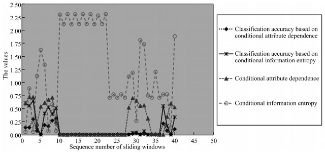
图 1 滑动窗口的大小为10 000, 且相邻窗口之间没有重复
Fig. 1 The size of sliding windows is 10 000 without repeat
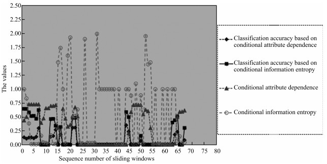
图 2 滑动窗口的大小为5 000, 且相邻窗口之间没有重复
Fig. 2 The size of sliding windows is 5 000 without repeat
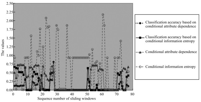
图 3 滑动窗口的大小为5 000, 且相邻窗口之间有10 %的重复
Fig. 3 The size of sliding windows is 5 000 with 10 % repeat
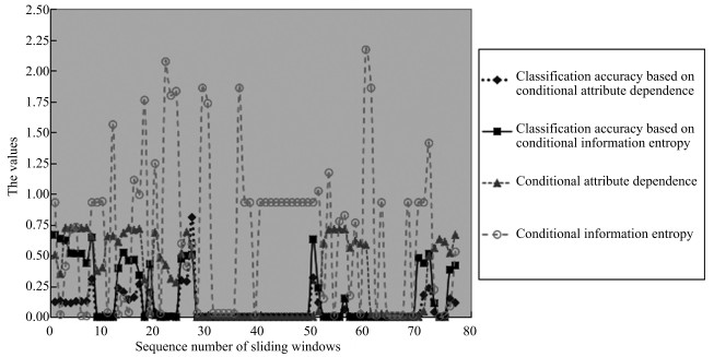
图 4 滑动窗口的大小为10 000, 且相临窗口之间有10 %的重复
Fig. 4 The size of sliding windows is 10 000 with 10 % repeat
表 1 决策子系统DT1
Table 1 A decision subsystem DT1
U1 a b c d x1 0 0 1 1 x2 1 1 0 1 x3 0 1 0 0 x4 1 1 0 1  下载: 导出CSV
表 2 决策子系统DT2
Table 2 A decision subsystem DT2
U2 a b c d y1 0 1 0 0 y2 1 1 0 1 y3 1 1 0 1 y4 0 1 0 0 y5 1 2 0 0 y6 1 2 0 1
下载: 导出CSV
-
[1] Babcock B, Babu S, Datar M, Motwani R, Widom J. Models and issues in data stream systems. In:Proceedings of the 21st ACM SIGMOD-SIGACT-SIGART Symposium on Principles of Database Systems. Madison, Wisconsin, USA:ACM, 2002. 1-16 [2] 王涛, 李舟军, 颜跃进, 陈火旺.数据流挖掘分类技术综述.计算机研究与发展, 2007, 44(11):1809-1815 http://d.old.wanfangdata.com.cn/Periodical/jsjyjyfz200711001Wang Tao, Li Zhou-Jun, Yan Yue-Jin, Chen Huo-Wang. A survey of classification of data streams. Journal of Computer Research and Development, 2007, 44(11):1809-1815 http://d.old.wanfangdata.com.cn/Periodical/jsjyjyfz200711001 [3] 徐文华, 覃征, 常扬.基于半监督学习的数据流集成分类算法.模式识别与人工智能, 2012, 25(2):292-299 doi: 10.3969/j.issn.1003-6059.2012.02.016Xu Wen-Hua, Qin Zheng, Chang Yang. Semi-supervised learning based ensemble classifier for stream data. Pattern Recognition and Artificial Intelligence, 2012, 25(2):292-299 doi: 10.3969/j.issn.1003-6059.2012.02.016 [4] Lu N, Zhang G Q, Lu J. Concept drift detection via competence models. Artificial Intelligence, 2014, 209:11-28 doi: 10.1016/j.artint.2014.01.001 [5] Domingos P, Hulten G. Mining high-speed data streams. In:Proceedings of the 6th ACM SIGKDD International Conference on Knowledge Discovery and Data Mining. Boston, Massachusetts, USA:ACM, 2002. 71-80 [6] Hulten G, Spencer L, Domingos P. Mining time-changing data streams. In:Proceedings of the 7th ACM SIGKDD International Conference on Knowledge Discovery and Data Mining. San Francisco, California, USA:ACM, 2001. 97-106 [7] 孙岳, 毛国君, 刘旭, 刘椿年.基于多分类器的数据流中的概念漂移挖掘.自动化学报, 2008, 34(1):93-97 http://www.aas.net.cn/CN/abstract/abstract16029.shtmlSun Yue, Mao Guo-Jun, Liu Xu, Liu Chun-Nian. Mining concept drifts from data streams based on multi-classifiers. Acta Automatica Sinica, 2008, 34(1):93-97 http://www.aas.net.cn/CN/abstract/abstract16029.shtml [8] Wang H X, Fan W, Yu P S, Han J W. Mining concept-drifting data streams using ensemble classifiers. In:Proceedings of the 9th ACM SIGKDD International Conference on Knowledge Discovery and Data Mining. Washington, D.C., USA:ACM, 2003. 226-235 [9] Li P P, Wu X D, Hu X G, Wang H. Learning concept-drifting data streams with random ensemble decision trees. Neurocomputing, 2015, 166:68-83 doi: 10.1016/j.neucom.2015.04.024 [10] 张明卫, 朱志良, 刘莹, 张斌.一种大数据环境中分布式辅助关联分类算法.软件学报, 2015, 26(11):2795-2810 http://d.old.wanfangdata.com.cn/Periodical/rjxb201511005Zhang Ming-Wei, Zhu Zhi-Liang, Liu Ying, Zhang Bin. Distributed assistant associative classification algorithm in big data environment. Journal of Software, 2015, 26(11):2795-2810 http://d.old.wanfangdata.com.cn/Periodical/rjxb201511005 [11] Bifet A, Holmes G, Pfahringer B, Kirkby R, Gavaldá R. New ensemble methods for evolving data streams. In:Proceedings of the 15th ACM SIGKDD International Conference on Knowledge Discovery and Data Mining. Paris, France:ACM, 2009. 139-148 [12] Gao J, Fan W, Han J W, Yu P S. A general framework for mining concept-drifting data streams with skewed distributions. In:Proceedings of the 2007 SIAM International Conference on Data Mining. Minnesota, USA:SIAM, 2007. [13] Widmer G, Kubat M. Effective learning in dynamic environments by explicit context tracking. In:Proceedings of the 1993 European Conference on Machine Learning. Vienna, Austria:Springer, 1993. 227-243 [14] 柴玉梅, 周驰, 王黎明.数据流上概念漂移的检测和分类.小型微型计算机系统, 2011, 32(3):421-425 http://d.old.wanfangdata.com.cn/Periodical/xxwxjsjxt201103008Chai Yu-Mei, Zhou Chi, Wang Li-Ming. Detecting concept drift and classifying data streams. Journal of Chinese Computer Systems, 2011, 32(3):421-425 http://d.old.wanfangdata.com.cn/Periodical/xxwxjsjxt201103008 [15] Pawlak Z. Rough sets. International Journal of Computer and Information Sciences, 1982, 11(5):341-356 doi: 10.1007/BF01001956 [16] 张清华, 薛玉斌, 王国胤.粗糙集的最优近似集.软件学报, 2016, 27(2):295-308 http://d.old.wanfangdata.com.cn/Periodical/rjxb201602008Zhang Qing-Hua, Xue Yu-Bin, Wang Guo-Yin. Optimal approximation sets of rough sets. Journal of Software, 2016, 27(2):295-308 http://d.old.wanfangdata.com.cn/Periodical/rjxb201602008 [17] 王国胤. Rough集理论与知识获取.西安:西安交通大学出版社, 2001.Wang Guo-Yin. Rough Set Theory and Knowledge Acquisition. Xi'an:Xi'an Jiaotong University Press, 2001. [18] 邓大勇, 陈林.并行约简与F-粗糙集.云模型与粒计算.北京:科学出版社, 2012. 210-228Deng Da-Yong, Chen Lin. Parallel reducts and F-rough sets. Cloud Model and Granular Computing. Beijing:Science Press, 2012. 210-228 [19] 陈林. 粗糙集中不同粒度层次下的并行约简及决策[硕士学位论文], 浙江师范大学, 中国, 2013.Chen Lin. Parallel Reducts and Decision in Various Levels of Granularity [Master thesis], Zhejiang Normal University, China, 2013. [20] Cao F Y, Huang J Z. A concept-drifting detection algorithm for categorical evolving data. In:Proceedings of the 17th Pacific-Asia Conference on Knowledge Discovery and Data Mining. Gold Coast, Australia:Springer, 2013. 485-496 [21] 邓大勇, 裴明华, 黄厚宽. F-粗糙集方法对概念漂移的度量.浙江师范大学学报(自然科学版), 2013, 36(3):303-308 doi: 10.3969/j.issn.1001-5051.2013.03.012Deng Da-Yong, Pei Ming-Hua, Huang Hou-Kuan. The F-rough sets approaches to the measures of concept drift. Journal of Zhejiang Normal University (Natural Sciences), 2013, 36(3):303-308 doi: 10.3969/j.issn.1001-5051.2013.03.012 [22] 邓大勇, 徐小玉, 黄厚宽.基于并行约简的概念漂移探测.计算机研究与发展, 2015, 52(5):1071-1079 http://d.old.wanfangdata.com.cn/Periodical/jsjyjyfz201505009Deng Da-Yong, Xu Xiao-Yu, Huang Hou-Kuan. Concept drifting detection for categorical evolving data based on parallel reducts. Journal of Computer Research and Development, 2015, 52(5):1071-1079 http://d.old.wanfangdata.com.cn/Periodical/jsjyjyfz201505009 [23] 苗夺谦, 胡桂荣.知识约简的一种启发式算法.计算机研究与发展, 1999, 36(6):681-684 http://d.old.wanfangdata.com.cn/Periodical/jsjyjyfz199906006Miao Duo-Qian, Hu Gui-Rong. A heuristic algorithm for reduction of knowledge. Journal of Computer Research and Development, 1999, 36(6):681-684 http://d.old.wanfangdata.com.cn/Periodical/jsjyjyfz199906006 [24] 王国胤, 于洪, 杨大春.基于条件信息熵的决策表约简.计算机学报, 2002, 25(7):759-766 doi: 10.3321/j.issn:0254-4164.2002.07.013Wang Guo-Yin, Yu Hong, Yang Da-Chun. Decision table reduction based on conditional information entropy. Chinese Journal of Computers, 2002, 25(7):759-766 doi: 10.3321/j.issn:0254-4164.2002.07.013 [25] 杨明.决策表中基于条件信息熵的近似约简.电子学报, 2007, 35(11):2156-2160 doi: 10.3321/j.issn:0372-2112.2007.11.023Yang Ming. Approximate reduction based on conditional information entropy in decision tables. Acta Electronica Sinica, 2007, 35(11):2156-2160 doi: 10.3321/j.issn:0372-2112.2007.11.023 [26] 邓大勇, 薛欢欢, 苗夺谦, 卢克文.属性约简准则与约简信息损失的研究.电子学报, 2017, 45(2):401-407 doi: 10.3969/j.issn.0372-2112.2017.02.019Deng Da-Yong, Xue Huan-Huan, Miao Duo-Qian, Lu Ke-Wen. Study on criteria of attribute reduction and information loss of attribute reduction. Acta Electronica Sinica, 2017, 45(2):401-407 doi: 10.3969/j.issn.0372-2112.2017.02.019 -

 下载:
下载:

计量
- 文章访问数: 2110
- HTML全文浏览量: 281
- PDF下载量: 572
- 被引次数: 0
