

A Master-slave Cross-coupled Iterative Learning Control for Repetitive Tracking of Nonlinear Contours in Multi-axis Precision Motion Systems
-
摘要: 针对多轴运动系统非线性轮廓的重复跟踪,传统时域交叉耦合迭代学习控制器(Cross-coupled iterative learning control,CCILC)的设计,各轴间的耦合算子计算精度要求高,计算效率低.本文提出一种主从交叉耦合迭代学习控制方法.基于主从控制设计方法,主动轴采用时域CCILC,从动轴采用位置域交叉耦合迭代学习控制(Position domain CCILC,PDCCILC).保证各轴间运动同步性,同时减轻对耦合算子精确性的依赖.因而可以引入轮廓误差矢量法估算耦合算子提高计算效率.采用Lifting的系统时域矩阵展开方法对所提出的算法进行了稳定性分析和性能分析.基于一个两轴毫米级运动平台,三种典型非线性轮廓跟踪(即半圆、抛物线和螺旋线)的数值仿真和实验分析验证了所提出算法的有效性.Abstract: In traditional time domain cross-coupled iterative learning control (CCILC) design, the requirements of high calculation accuracy of coupling gains between axes and low computational efficiency restrict its application to nonlinear contour tracking in repetitive tasks. This paper presents a master-slave cross-coupled iterative learning control. Based on the master-slave control design concept, the master motion axis applies time domain CCILC, while the slave motion axis adopts position domain CCILC (PDCCILC). The proposed PDCCILC control can improve synchronization between axes as well as relieve the dependence on accuracy of coupling gains, therefore, the efficient contour error vector method can be adopted to estimate the coupling gains. both stability and performance analyses are conducted using the lifted system representation method. Simulation and experimental results of the three typical nonlinear contour tracking cases (i.e., semi-circle, parabola and spiral) with a two-axis micro-motion stage have demonstrated superiority and efficacy of the proposed controller.
-
肌电信号 (Electromyography, EMG) 在激发肌肉活动时产生, 是一种重要的运动生物力学信息, 与人体的期望动作直接相关, 尤其是表面肌电信号以其无创伤测量、易提取的优点, 成为感知人体运动意图的理想信息源, 广泛地应用于外骨骼助行机器人、假肢等下肢康复辅具控制[1-3].
通过EMG可以在未做出动作前获取主动运动意图, 相对于仅仅采集姿态、速度等运动力学信息的传统方法具有明显优势[4-5].在肌电控制下肢康复辅具过程中, 为了得到更好的模式识别结果, 确定能更好地区分各模式的肌电信号采集位置非常重要.
虽然下肢表面EMG蕴含足够的信息以表达患者应对运动模式更替的意愿, 但是目前肌电电极放置位置并没有成熟的理论依据和统一标准, 缺乏对不同运动模式过程中全面动态EMG的变化与联系的理论层次解读.
通常是基于解剖学的已有知识, 通过对下肢各主要肌群进行统计学分析或实验[6-9], 分析比较各肌群的EMG关联关系.例如, 佟丽娜等[6]利用健康个体单侧8块主要肌群的表面EMG识别下肢踏车、行走和椭圆运动模式, 通过分析8路信号的平均相似度及标准差, 将8块肌肉减少到3块, 最终准确率高达91.67 %.又如佘青山等[7]通过大量反复实验, 选用4块大腿肌肉作为下肢EMG的来源, 将一个步态周期细分为支撑前期、支撑中期等5种运动模式. He等[8]则通过分析坐下、蹲、上下楼及行走过程中的单侧13块肌肉, 确定各种运动过程中的主要作用肌群.虽然以上肌肉采集位置的确定方法已经涵盖了下肢的大部分肌群, 取得了较好的研究成果, 但是仍未覆盖整个下肢表面.随着肌群个数的增加, 统计学分析或实验的工作量将急剧增加, 因此对整个下肢表面的EMG进行综合分析与比较是不现实的, 这就使得当前的运动模式识别结果有可能不是最理想的, 有可能通过肌电位置优化进一步提高识别效果.
另一方面, 为了全面、深入了解不同运动模式中的电生理过程, 对运动模式做出准确的识别, 需要采集多个通道的EMG [10-11], 获取全面的动态肌电信息.但是肌肉之间又存在着严重的相似性, 需要通过分析各通道间的耦合关系最大限度地减少电极数目.
常用主元分析法 (Principal component analysis, PCA) 根据各特征参数的贡献率降低特征参数维数[12].虽然对于特定信号效果很好, 但是对各肌肉贡献率描述中无法体现时间信息.由于各肌肉在每个运动阶段的作用不同, 贡献率也不同, 可能两块肌电特性相似的肌肉贡献率都很大, 也可能贡献率低的肌肉在某阶段运动描述中必不可少.所以, 简单的PCA分析并不能完全揭示下肢肌肉的神经动力学关系.
复杂网络理论作为一种研究复杂系统动力学的有效方法, 首先由Watts等[13]和Barabási等[14]提出, 复杂网络的局部和全局特性能够清晰地刻画组成复杂系统的不同元素之间的相互关系和信息流动过程, 在大脑功能认识[15-16]、蛋白质互相作用网络[17]、网络搜索、传染病控制及突发事件预报等方面提供了很好的科学理解和定量分析.尤其是脑功能网络, 是复杂网络理论在神经科学中的重要应用, 已经得到很多重要成果, 并为揭示脑疾病的病理机制提供了新思路[15-16].
本文将复杂网络理论应用于下肢EMG分析, 在下肢肌肉表面选取90个EMG采集点作为节点, 构建下肢肌肉功能网络; 通过网络拓扑属性分析[18-19], 证明下肢肌肉功能网络的小世界属性, 总结其统计学特点; 在网络层面分析不同运动模式过程中的拓扑结构差异和肌肉功能共异性, 深入分析不同运动模式状态下肌肉功能结构的共异性, 确定与运动模式更替关联度大的肌群和电极位置.下肢肌肉功能网络构建与分析将揭示下肢EMG与运动模式更替之间的关系, 为运动模式识别与调控提供可靠的理论支持.
1. 下肢肌肉功能网络构建
依次记录两侧下肢的整个肌肉系统在3种运动模式 (平地行走、上楼梯和下楼梯) 过程中的表面EMG, 构建下肢肌肉功能网络, 深入讨论各采集点与模式切换间的关系.
定义1.一个无向无权网络$G=(V, E)$具有$n$个节点和$m$条边, 其顶点集为$V=\{V_1, \cdots, V_n \}$, 边集合为
$ E= \left\{ {E_j|E_j\in V\times V, \ j =1, \cdots, m} \right\} $
(1) 定义2.构造网络$G$的邻接矩阵$A=(A_{ij})_{n\times n}$
$ {A_{ij}} = \left\{ {\begin{array}{*{20}{l}} {1, }&{{\rm{若}}\left| {{C_{ij}}} \right| \ge TH}\\ {0, }&{若\left| {{C_{ij}}} \right| < TH} \end{array}} \right. $
(2) 其中, $C_{ij}$为节点$i$和节点$j$间的Pearson系数, $TH$为阈值.如果$A_{ij}=1$, 表示节点$i$与$j$之间有连边, 否则$A_{ij}=0$, 表示节点$i$与$j$之间无连边.
1.1 定义网络节点
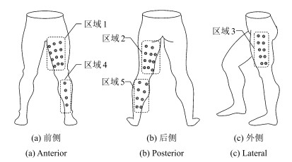
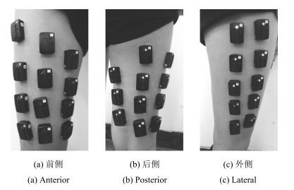
将人体下肢与运动模式变化相关的肌肉系统分为10个区域, 左腿和右腿的EMG采集点分布情况相同, 以左侧下肢为例, 如图 1所示, 左侧下肢分为5个区域.在两侧下肢肌肉表面均匀选取$n=90$个EMG采集点作为节点, 记作$V1$ $\sim$ $V90$, 如表 1所示.
表 1 肌电电极分区与分布情况Table 1 The partition and distribution of EMG electrodes区域 个数 节点 名称 位置 分布情况 1 12 V01~V12 LTF1~LTF12 左侧大腿前侧 四排三列 2 11 V13~V23 LTP1~LTP12 左腿大腿后侧 三列 (三排一列+四排两列) 3 10 V24~V33 LTL1~LTL10 左腿大腿外侧 五排两列 4 4 V34~V37 LCF1~LCF4 左侧小腿前侧 纵向排列 5 8 V38~V45 LCP1~LCP8 左腿小腿后侧 四排两列 6 12 V46~V57 RTF1~RTF12 右侧大腿前侧 四排三列 7 11 V58~V68 RTP1~RTP12 右腿大腿后侧 三列 (三排一列+四排两列) 8 10 V69~V78 RTL1~RTL10 右腿大腿外侧 五排两列 9 4 V79~V82 RCF1~RCF4 右侧小腿前侧 纵向排列 10 8 V83~V90 RCP1~RCP8 右腿小腿后侧 四排两列 1.2 基于移动窗的EMG分段
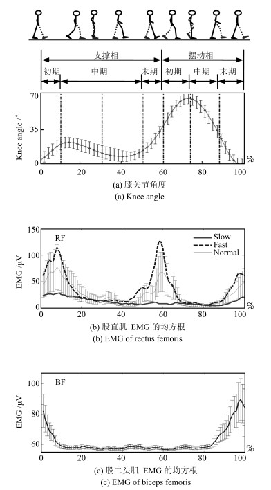
相对于上肢而言, 下肢的运动更具有周期性特点, 一个步态周期定义为从脚跟着地开始到同侧脚跟再次着地结束 (图 2 (a)), 可以分为支撑相和摆动相两个部分.采集不同步速下$(Fast: 1.75 {\rm m/s}$; $Normal:$ $1.25 {\rm m/s}$; $Slow: 0.75 {\rm m/s})$股直肌的表面EMG, 计算其均方根, 如图 2 (b) 所示, 在整个运动周期内, EMG呈周期性变化, 股直肌在支撑相末期至摆动相中期、摆动相末期至支撑相中期两阶段起作用, 肌电信号比较活跃, 并随步速增加而增加.而股二头肌EMG的均方根 (图 2 (c)) 在摆动相中末期、首次触地至承重反应结束过程中起作用.
由于数据采集点来自双侧下肢, 所以仅记录并分析支撑相 (从脚跟着地开始到同侧脚脚尖离地结束) 过程的EMG.
选取采集点支撑相的$i$的EMG样本数据, 采用移动时间窗进行处理, 将其分为$w$段信号, 进行去除零点漂移、滤波等预处理后, 通过提取时间窗内的特征向量, 用于下肢肌肉功能网络构建.为了便于兼顾过程的时变性和信息的完整性, 选择移动窗的窗口长度$h=150 \rm ms$, 步长$S=50 \rm ms$, 采样频率2 000 Hz.
1.3 特征提取
选择EMG采集点$i$ $(i=1, 2, \cdots, n)$的第$t$ $(t$=$1, 2, \cdots, w)$时间窗, 设时间窗内的$h$个EMG数据为$x_{it}=\left\{x_{it}(1), x_{it}(2), \cdots, x_{it}(h)\right\}$, 计算$x_{it}$的8个时域和频域特征向量, 包括最大值$(Ma_{it})$、绝对值平均$(Mav_{it})$、标准差$(Std_{it})$、均方根$(RMS_{it})$、能量$(V_{it})$、平均功率频率$(MPF_{it})$、中值频率$(MFP_{it})$、峰值频率$(F_{it})$.
$ M{a_{it}} = \max \left\{ {{x_{it}}(1), {x_{it}}(2), \cdots, {x_{it}}(h)} \right\} $
(3) $ Ma{v_{it}} = \sum\limits_{q = 1}^h {\frac{{\left| {{x_{it}}(q)} \right|}}{h}} $
(4) $ St{d_{it}} = \sqrt {\sum\limits_{q = 1}^h {\frac{{{{\left[{{x_{it}}(q)-{{\bar x}_{it}}} \right]}^2}}}{{h -1}}} } $
(5) 其中, $\overline{x}_i=\sqrt {\sum_{q=1}^h{x^{2}_{it}(q)/h}}$.
$ RM{S_{it}} = \sqrt {\sum\limits_{q = 1}^h {\frac{{x_{it}^2(q)}}{h}} } $
(6) $ {V_{it}} = \sum\limits_{q = 1}^h {\left| {{x_{it}}} \right|} $
(7) $ MP{F_{it}} = \frac{{\int_0^\infty f \times {s_{it}}(f){\rm{d}}f}}{{\int_0^\infty {{s_{it}}} (f){\rm{d}}f}} $
(8) $ MF{P_{it}} = 0.5\int_0^\infty {{s_{it}}} (f){\rm{d}}f $
(9) $ {F_{it}} = \max \left[{{s_{it}}(f)} \right] $
(10) 其中, $s_{it}(f)$为功率谱密度函数.
比较发现, 增加时域或频域特征向量的个数对于复杂网络的连边影响很小.经过多次试验与对比, 选取绝对值平均$(Mav_{it})$、均方根$(RMS_{it})$、能量$(V_{it})$、中值频率$(MFP_{it})$四个特征值构建复杂网络.
提取EMG采集点$i$的第$t$时间窗的特征值, 构建矩阵$T_{it}$:
$ T_{it}=(Mav_{it}, RMS_{it}, V_{it}, MFP_{it}) $
(11) 其中, $i$表示EMG采集点的标号.
EMG采集点$i$的特征值构建$w\times 4$的矩阵$T_i$:
$ T_i=(Mav_i, RMS_i, V_i, MFP_i) $
(12) 对矩阵$T_i$进行归一化处理, 得到$T_i'$:
$ T'_i=(mav_i, rms_i, v_i, mfp_i) $
(13) 所有EMG采集点的每个特征向量构成一个$w$ $\times$ $n$的特征矩阵$M_p$ $(p=1, 2, 3, 4)$, $M_1=mav$, $M_2$ $=$ $rms$, $M_3=v$, $M_4=mfp.$
1.4 连边的生成
计算特征矩阵$M_p$的任意两列向量间的Pearson系数
$ {C_{pij}} = \frac{{\sum\limits_{t = 1}^w {\{ [{M_{pi}}(t)-\langle {M_{pi}}\rangle] \times [{M_{pj}}(t)-\langle {M_{pj}}\rangle]\} } }}{{\sqrt {\sum\limits_{t = 1}^w {{{[{M_{pi}}(t)-\langle {M_{pi}}\rangle]}^2}} } \times \sqrt {\sum\limits_{t = 1}^w {{{[{M_{pj}}(t)-\langle {M_{pj}}\rangle]}^2}} } }} $
(14) 其中, $C_{pij}$为肌电采集点$i$和肌电采集点$j$间的第$p$个特征值的Pearson系数, $M_{pi}$和$M_{pj}$分别为第$p$个特征值的矩阵$M_p$的第$i$列和第$j$列$(i=1, 2$, $\cdots, n$, $j=1, 2, \cdots, n)$, $M_{pi}(t)$和$M_{pj}(t)$分别为向量$M_{pi}$和$M_{pj}$的第$t$行元素, $\langle M_{pi}\rangle$和$\langle M_{pj}\rangle$分别为向量$M_{pi}$和$M_{pj}$的$w$个元素的平均值.
肌电采集点$i$和肌电采集点$j$间的Pearson系数
$ C_{ij}=\frac{1}{{4}}{\sum\limits_{p=1}^4{C_{pij}}} $
(15) 计算$n$个EMG采集点间的Pearson系数构成一个对称矩阵$C=(C_{ij})_{n\times n}$, 评价各肌电采集点间的相关程度.
构建下肢EMG网络, 把每个采集位置看作一个节点, 分析任意两点间的相关性, 如果两点间的相关系数大于给定阈值$TH$, 则认为两点间有功能性连接, 各采集点间的连接关系代表网络连边.
如果阈值取得过小, 那么可能建立起一个完全连通的下肢肌肉功能网络图, 对于肌电电极采集点分析没有任何意义; 如果阈值取得过大, 则可能建立一个过于稀疏的网络, 致使大量有用信息丧失, 所以阈值选择对于网络构建至关重要.
2. 网络拓扑属性分析
2.1 阈值确定与稀疏度
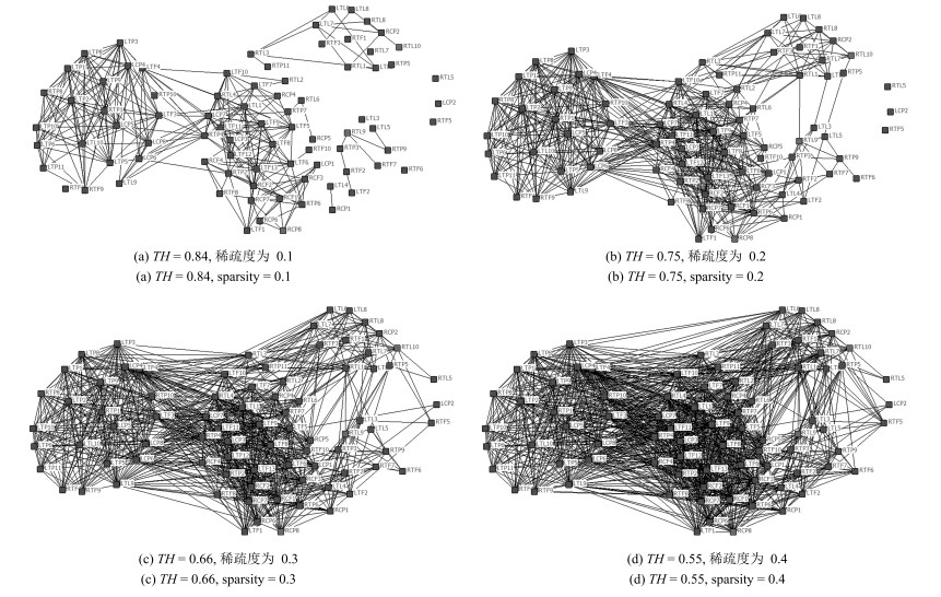
选取合适的阈值并在连接强度大于阈值的节点间建立连接边.阈值的选择直接影响邻接矩阵边的生成和下肢肌肉功能网络的拓扑结构, 不同的阈值会导致网络规模和网络结构发生明显变化, 以下楼梯为例, 如图 3所示, 构建不同阈值$TH$的下肢肌肉功能网络, 分析得到阈值$TH$与稀疏度$S_p$间的函数关系.
$ S_p=-0.72 TH+0.674 $
(16) 即阈值与网络稀疏度成反比关系, 阈值越大, 网络越稀疏, 相应的节点之间的连边越少, 各节点之间的联系较分散; 反之, 阈值越小, 网络越密集, 相应节点之间的连边越多, 各节点之间联系越紧密.
式 (16) 中, 在阈值$TH=0.75$时, 网络稀疏度为0.2, 如图 3 (b) 所示, 网络可以分为两个社团结构; 而当阈值过大时, 稀疏度过小, 如图 3 (a) 所示, 虽然也可看大体的社团分布情况, 但是会出现9个孤立点, 致使有些连接被忽视; 当阈值过小时, 稀疏度较大, 如图 3 (c) 和图 3 (d) 所示, 过于密集的网络结构致使社团结构不明显, 结构趋向于随机.
2.2 邻接矩阵
计算两两肌电采集位置间的Pearson系数, 利用合适的阈值, 得到$90\times90$的邻接矩阵.当阈值$TH$ $=$ $0.75$时, 构建三种运动模式 (平地、上楼和下楼) 的邻接矩阵, 如图 4所示.其中, 横坐标和纵坐标表示EMG采集位置的节点序号, 黑色表示两点之间有连接, 白色表示无连接.三种模式相比, 节点间相关程度高的节点均不相同.
由图 4 (a) 知, 平地模式中各节点间的联系比较紧密, 尤其是节点$10$ $\sim$ $72$间的大部分节点间的关系都比较紧密; 而上下楼梯模式的节点间的相关程度较低, 如图 4 (c) 所示, 下楼梯模式下, 只有节点$1$ $\sim$ $15$之间、节点$21$ $\sim$ $33$间的相关程度较高.所以, 可以利用所得的邻接矩阵构建下肢肌肉功能网络, 通过分析网络的拓扑属性确定与运动模式更替关系密切的EMG采集位置.
2.3 特征参数
利用图论方法, 计算节点度 (Node degree)、平均度 (Average degree)、聚类系数 (Clustering coefficient)、平均路径长度 (Average path length)、介数 (Betweenness) 等特征参数[13-19], 进一步分析网络的连接规律.
2.3.1 节点度ki
节点度${ k}_i$表示与节点$i$相关联的边的条数, 反映这个节点在网络中的活跃度, 和节点对其相邻节点的影响力.节点度越大, 节点对其相邻节点的重要度贡献越大, 在网络中起着更重要的作用.
$ k_i=\sum\limits_{j=1}^n{A_{ij}} $
(17) 2.3.2 平均度$\langle \boldsymbol{k}\rangle $
网络的平均度$ \langle { k} \rangle$表示整个网络中所有节点度的平均值.
$ \langle k\rangle=\frac{1}{{N}}\sum\limits_{i, j=1}^n{A_{ij}} $
(18) 2.3.3 聚类系数$\boldsymbol{CC}_{\boldsymbol{i}}$
聚类系数${ {CC}}_{i}$表示节点$i$聚集程度的系数, 是描述网络集团化的重要指标.
$ CC_i=\frac{2e_i}{{k_i({k_i}-1)}} $
(19) 其中, $e_i$为节点$i$与相连的$k_i$个节点间实际存在的边数.
2.3.4 平均路径长度$\boldsymbol{L}$
平均路径长度${ L}$表示任意两个节点之间距离的平均值.
$ L={\frac{n}{{K}}}f(nKp) $
(20) 其中, $f (\cdot)$为普适标度函数, $K$为平均节点度, $p$为重连概率.
2.3.5 介数$\boldsymbol{B}_{\boldsymbol{i}}$
介数${ B}_{i}$表示网络中所有的最短路径中, 经过该节点的数量, 反映了节点的影响能力, 因此介数大的点在网络信息传输中起关键作用.
$ B_i=\sum\limits_{j, m\in V, i\neq j\neq m}{\frac{\sigma_{j.m}(i)}{{\sigma_{j, m}}}} $
(21) 其中, $\sigma_{j, m}$表示节点$j$和节点$m$间最短路径总数, $\sigma_{j, m}(i)$则表示经过节点$i$且连接节点$j$和节点$m$的最短路径总数.
网络介数分析了网络中节点对间沿着最短路径传输信息的控制能力, 如果两个节点之间没有路径, 或者一个节点没有位于另外两个节点之间的任何一条最短路径上, 则说明该节点对另外两个节点之间的信息传输没有直接控制能力.
3. 实验结果及分析
3.1 数据采集
利用Delsys公司的Trigno Wireless System无线采集系统, 记录3种行走模式 (平地、上楼和下楼, 其中楼梯台阶高度为15 cm) 在支撑相的下肢表面EMG, 如图 5所示.受试者具体情况如表 2所示, 均无下神经肌肉或肌肉骨骼方面疾病.
表 2 受试者信息Table 2 The information of subjects实验对象 性别 年龄 身高 (cm) 体重 (kg) S1 女 24 165 48 S2 女 24 170 54 S3 女 45 162 65 S4 女 65 155 73 S5 男 23 172 80 S6 男 27 180 95 S7 男 42 175 70 S8 男 62 170 72 3.2 下肢肌肉功能网络构建
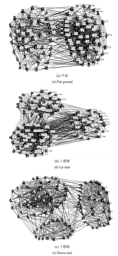
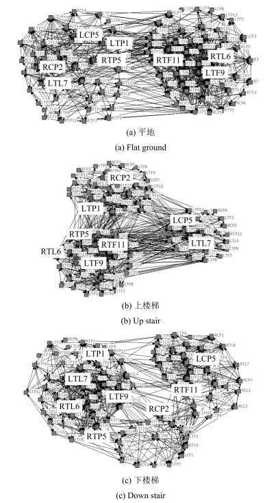
对每个节点采集的EMG进行预处理, 提取4个时频域特征向量 (绝对值平均、均方根、能量、中值频率).利用每个节点的特征向量计算皮尔森系数, 选取适当的阈值, 得到邻接矩阵, 其中0代表两个节点之间没有连边, 1代表两个节点之间有连边.利用netdraw软件画出各运动模式的功能网络, 如图 6所示.
由图 6可知, 不同运动模式下的复杂网络及作用节点均具有明显差异.其中, 平地模式连边数最多, 说明各节点间的相似程度较高, 在平地运动时, 存在相似电运动的电极位置较多.上楼和下楼模式的功能网络连边数相对少一些, 社团结构比较明显, 说明在两种模式过程中, 存在一些节点位置的EMG时域特性比较特殊, 与其他节点的相似程度比较低, 分析并确定这些特殊的、具有显著差异的节点, 有助于识别运动模式间的更替.
3.3 小世界特性
经过大量的实验证明[13-19], 绝大部分复杂网络都具有小世界特性, 规则网络和随机网络都无法再现许多实际网络具有的小世界特征.小世界网络既不像随机网络具有较短的平均路径和较低的聚类系数, 也不像规则网络具有较长的平均路径和较高的聚类系数, 而是介于两者之间.
为了证明下肢肌肉功能网络的小世界特性, 根据式 (18) $\sim$ (20) 计算三种运动模式的复杂网络特性, 包括网络节点数$n$, 网络节点的平均度$\langle k\rangle$, 总连边数$edges$, 聚类系数$CC$, 平均路径长度$L$, 对应的规则网络的聚类系数$C_{nc}$和平均路径长度$L_{nc}$, 对应的随机网络的聚类系数$C_{ER}$和平均路径长度$L_{ER}$.
计算小世界特性的指标如下:
$ \gamma =\frac{C}{{C_{ER}}} $
(22) $ \lambda =\frac{L}{{L_{ER}}} $
(23) $ \sigma =\frac{\gamma}{\lambda} $
(24) 只有当$\gamma>1$, $\lambda \approx 1$, $\sigma>1$同时满足时, 该网络才符合小世界网络特性.计算三种运动模式下复杂网络的主要特性参数, 如表 3所示.三种运动模式的复杂网络均符合$\gamma>1$, $\lambda \approx 1$, $\sigma>1$的小世界特性指标, 因此, 说明构建的下肢肌肉功能网络具有小世界的网络特性, 即任意两个节点间的距离都维持在一个相对较小的固定值, 可以通过分析网络的节点度、聚类系数等统计特征研究网络性质, 为分析下肢肌肉的协调工作机制提供新的方法.
表 3 三种模式复杂网络的小世界特性参量统计Table 3 Three models of complex networks of small world characteristic parameter statistics运动模式 $n$ $langlekrangle$ $edges$ $CC$ $L$ $C_{nc}$ $L_{nc}$ $C_{ER}$ $L_{ER}$ $gamma=C/{C_{ER}}$ $lambda=L/{L_{ER}}$ $sigma=gamma/lambda$ 平地 90 30.0 2487 0.8883 1.7857 0.7241 1.3833 0.3659 1.2992 2.4277 1.3745 1.7662 上楼梯 90 13.1 1091 0.8874 2.3736 0.6880 3.1679 0.1598 1.7129 5.5532 1.3857 4.0075 下楼梯 90 16.1 1337 0.8318 2.0372 0.7003 2.5776 0.1963 1.5902 4.2374 1.2811 3.3076 3.4 阈值对网络统计特性的影响
阈值的选取对于复杂网络的构建尤为重要, 为了确定合适的阈值, 利用不同阈值构建下肢肌肉功能网络.由于复杂网络的稀疏度不能超过0.5 [20], 所以阈值设定从0.5开始, 每次增加0.05, 直至0.95.以下楼梯模式为例, 计算各网络的稀疏度$S_p$、平均度$\langle k\rangle$及聚类系数$CC$, 如表 4所示.
表 4 不同阈值下的网络统计特性Table 4 Network statistical characteristics under different threshold$TH$ 稀疏度$S_p$ 平均度$langlekrangle$ 聚类系数$CC$ 0.5 0.4916 40.81 0.7527 0.55 0.4266 35.41 0.7665 0.6 0.3648 30.28 0.7708 0.65 0.3024 25.10 0.7899 0.7 0.2472 20.52 0.7945 0.75 0.1941 16.11 0.8318 0.8 0.1418 11.77 0.8250 0.85 0.0910 7.55 0.8193 0.9 0.0565 4.69 0.7194 0.95 0.0344 2.86 0.5770 由表 4可以看出, 下肢肌肉功能网络的平均度和稀疏度均与阈值成反比, 聚类系数则随着阈值增加呈现抛物线变化, 即会出现一个极大值点.聚类系数是描述一个复杂网络任意两节点之间互相关联的概率, 其值越大, 表示节点之间联系越紧密.所以选取聚类系数达到最大值 (0.8318) 时的阈值$TH$ $=$ $0.75$, 此时稀疏度为0.1941, 比较合适.
3.5 显著性差异
从控制信息传输的角度而言, 介数越高的节点其重要性也越大.分析三种运动模式 (平地、上楼和下楼) 的下肢肌肉功能网络, 计算节点的介数, 如表 5所示.
表 5 不同模式下节点介数特性统计Table 5 Node betweenness under different model排序 平地 下楼 上楼 1 RTL4h 280.1 LCP6h 1644.4 RCP4h 557.2 2 RTF9h 277.7 RTP6h 1473.8 RCP8h 366.5 3 RTL10h 267.0 RCP3h 1369.9 RCP6h 344.4 4 LTP5h 236.4 LTL4h 1304.2 RCP5h 327.2 5 RTF10h 208.8 RTP3h 1216.6 RTP6h 318.2 6 RTF7h 180.6 RCP2h 1212.6 LTP3h 301.6 7 LTF10h 161.4 RTL1h 1198.6 RTF8h 287.5 8 LCP3h 151.1 RTL9h 1141.3 RTP3h 221.2 9 RTF1h 135.9 RTP2h 1048.7 RTP1h 218.5 10 LCP5h 128.4 RTL2h 932.4 RTL8h 193.0 由表 5可知, 不同运动模式下介数最大的节点完全不同, 说明在各种运动模式中的重要节点不同.另外, 各运动模式的介数最大值也不同, 平地为280.1, 上楼梯为557.2, 下楼梯更是高达1 644.4, 这是因为各种功能网络的节点间连接不同, 连边数量也有差异.同时, 节点对之间的传输频率不完全相同, 也并非所有的传输都是基于最短路径的.因此, 介数最大值存在明显差异, 下楼数据远高于上楼及平地 (P < 0.001), 上楼数据平均也高于平地数据 (P=0.009).
综合考虑所有肌电采集点的3个主要特性参数 (节点度$k_i$、聚类系数$CC_i$、介数$B_i$), 对上楼梯、下楼梯与平地进行组间差异分析, 并采用投票的方式选取出整个网络差异值最大的几个节点, 发现整个数据采集区域中共有8个采集点具有显著差异 (P < 0.05), 如表 6所示.
表 6 不同模式下节点介数特性统计Table 6 Node betweenness under different model排序 节点标号 位置 1 RTP5 右腿大腿后侧 2 LTP1 左腿大腿后侧 3 LTL7 左腿大腿后侧 4 LTF9 左腿大腿前侧 5 RTL6 右腿大腿外侧 6 RCP2 右腿小腿后侧 7 LCP5 左腿小腿后侧 8 RTF11 右腿大腿前侧 在三种运动模式的下肢功能网络中 (阈值均为0.75) 标出8个具有显著差异的节点, 如图 7所示, 用连线图形象直观地展示了不同模式的重要节点连接关系.发现各点分布很均匀, 左右腿各4个, 其中大腿3个, 小腿1个.另外, 由于平地与上/下楼梯运动过程中, 主要是后侧肌肉工作方式有区别, 因此重要节点有4个位于人体后侧, 前侧和两侧分别2个, 分析结果与实际运动情况相吻合.
3.6 结果验证
利用表 7中列出的8个肌电采集位置 (单侧腿4个) 的表面EMG进行运动模式识别, 与常用各下肢肌肉肌腹中心位置[6-7]的表面EMG相比较.其中常用肌肉如下:
表 7 不同特征提取方法的模式识别比较Table 7 Comparison of pattern recognition based on different methods of feature extraction序号 单侧肌肉数目 肌肉采集点 识别率 (%) LDA SVM NN S1 12 大腿:RF, VL, BF, VM, ST, SM, AL, KTF小腿:TA, PL, GM, SM 78.1 82.3 80.2 S2 8 大腿:RF, VL, BF, VM, ST小腿:TA, GM, SM 91.4 93.1 92.2 S3 6 大腿:RF, VL, BF, VM小腿:TA, GM 95.6 97.6 97.3 S4 3 大腿:RF, VL小腿:SM[6] 84.4 85.7 86.4 S5 4 大腿:VM, SM, AL, KTF[7] 87.4 90.6 89.9 S6 4 下肢肌肉功能网络分析结果 95.3 98.4 97.9 1) 大腿肌肉:股直肌 (RF)、股外侧肌 (VL)、股二头肌 (BF)、股内侧肌 (VM)、半腱肌 (ST)、半膜肌 (SM)、长收肌 (AL)、阔筋膜张肌 (KTF);
2) 小腿肌肉:胫骨前肌 (TA)、腓骨长肌 (PL)、内侧腓肠肌 (GM)、比目鱼肌 (SM).
分别利用常用的线性判别分析 (Linear discriminant analysis, LDA)、支持向量机 (Support vector machine, SVM) 和神经网络 (Neural networks, NN), 对各种肌肉组合形式的采集点进行三种运动模式识别 (平地、上/下楼梯), 如表 7所示.
由表 7可知, 基于下肢肌肉功能网络选出的采集节点$S6$, 在模式识别中各种识别算法均可得到较好的识别结果, 能够满足下肢运动识别的需求.肌群的个数并非越多越好, 例如$S1$, 选择过多的与模式更替无关的肌群, 不仅无法提高识别效果, 还会大大降低识别精度.
虽然$S3$选择6组肌肉的情况也可以取得理想的识别效果, 但是所需电极数量将会增加, 人体两侧共需增加$2\times 2=4$个肌电电极, 将为信号的采集与处理带来不必要的麻烦.由于6组肌肉可以与网络选择的4组肌肉得到相近的识别效果, 说明6组肌肉中存在2组是冗余信息, 可以通过复杂网络分析有效地降低肌电采集个数.
另一方面, $S4$所选肌群虽然在下肢踏车、行走和椭圆运动模式取得了较好的识别结果[6], 但是并不适用于平地与上/下楼梯运动识别, 需要针对不同的识别目的, 进行大量的统计学分析进行筛选.由于$S5$只选择了大腿肌肉, 因此识别效果也欠佳, 重新的选择仍需大量的实验与分析.
综上所述, 基于下肢肌肉功能网络可以对运动相关肌肉的全面动态EMG进行综合分析, 确定与不同模式关联度大的肌群和电极放置位置, 为运动模式识别提供可靠的基础支持.
4. 结论
选取下肢主要肌肉表面的90个肌电采集位置作为节点, 通过分析各节点的表面EMG间的相关性, 构建下肢肌肉功能网络.在网络层面分析不同运动模式状态下的拓扑结构差异, 深入分析平地、上下楼梯三种模式中下肢肌肉功能网络的共异性, 最终确定了与运动模式更替关联度大的肌群和电极位置, 为下肢康复辅具中的肌电采集位置的确定提供了理论依据.
此方法可以推广到其他肌电控制康复辅具, 尤其是肌电假肢膝关节[21], 由于大腿截肢, 部分肌肉被切除, 原有的机能受到了很大的破坏, 残肢肌肉无法像健康人一样有力的收缩, 不能完全参考健肢肌肉放置电极.可以构建残肢肌肉功能网络, 确定与运动模式更替关联度更大的肌电采集位置.
下肢肌肉功能网络的研究中, 还有很多亟待解决的问题, 包括社团探寻、加权网络及动态网络的构建及分析等.随着研究的深入, 基于复杂网络的下肢肌电分析方法必将为下肢康复辅具控制提供更多的理论支持.
-
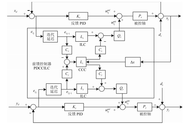
图 3 融合反馈PID和前馈PDCCILC的控制结构
Fig. 3 Combined feedback PID and feedforward PDCCILC control structure
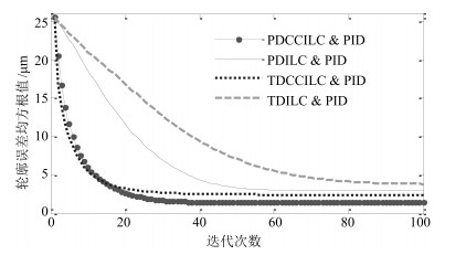
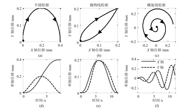
图 7 半圆轮廓跟踪均方根轮廓误差的仿真结果(RMS)
Fig. 7 RMS contour error versus iteration for the semi-circle contour in the simulations

图 8 半圆轮廓跟踪的稳态仿真结果
Fig. 8 Steady tracking results of the semi-circle contour in the simulations
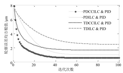
图 9 抛物线轮廓跟踪的仿真均方根轮廓误差(RMS)
Fig. 9 RMS contour error versus iteration for the semi-circle contour in the simulations

图 10 抛物线轮廓跟踪的稳态仿真结果
Fig. 10 Steady tracking results of the parabolic contour in the simulations
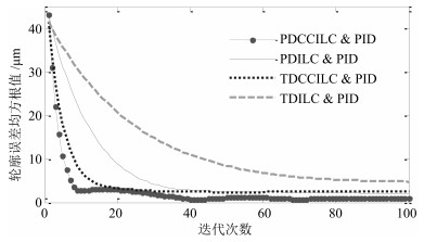
图 11 螺旋线轮廓跟踪的仿真均方根轮廓误差(RMS)
Fig. 11 RMS contour error versus iteration for the spiral contour in the simulations

图 12 螺旋线轮廓跟踪的稳态仿真结果
Fig. 12 Steady tracking results of the spiral contour in the simulations

图 13 半圆轮廓跟踪的实验均方根轮廓误差(RMS)
Fig. 13 RMS contour error versus iteration for the semi-circle contour in the experiments
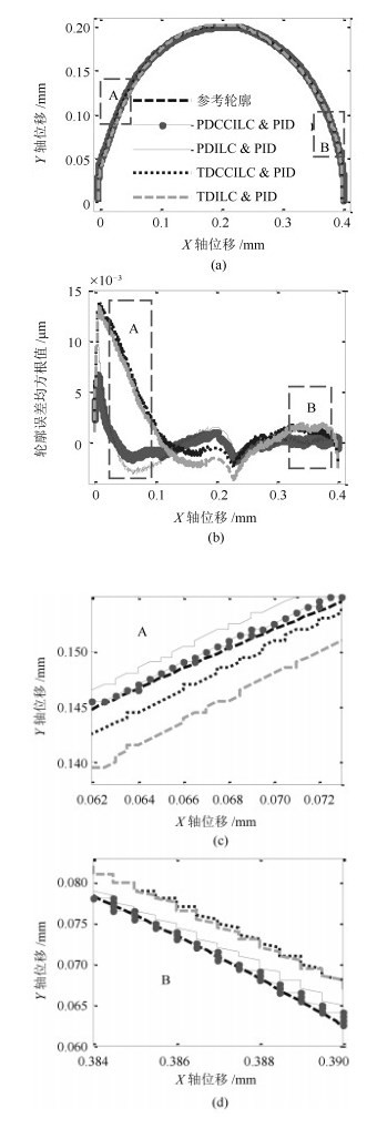
图 14 半圆轮廓跟踪的实验结果
Fig. 14 Tracking results of the semi-circle contour in the experiments
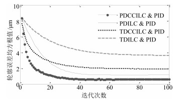
图 15 抛物线轮廓跟踪的实验均方根轮廓误差(RMS)
Fig. 15 RMS contour error versus iteration for the parabolic contour in the experiments
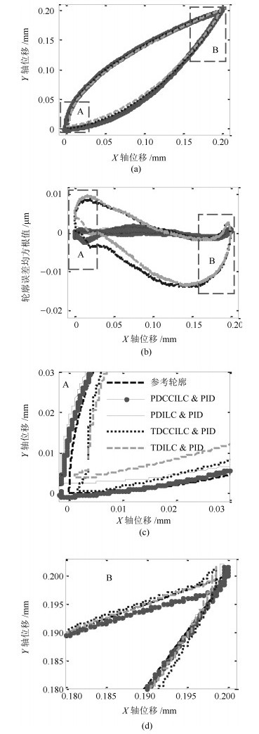
图 16 抛物线轮廓跟踪的实验结果
Fig. 16 Tracking results of the parabolic contour in the experiments

图 17 螺旋线轮廓跟踪的实验均方根轮廓误差(RMS)
Fig. 17 RMS contour error versus iteration for the spiral contour in the experiments
表 1 控制器参数
Table 1 Controller parameters
控制器 增益 ${K_p}$ ${K_i}$ ${K_d}$ PID 3 1 0 ILC 0.3 0.1 0.1 CCC 1 0.5 0  下载: 导出CSV
表 2 单调收敛的计算结果
Table 2 Computational results of monotonic convergence
控制器 $\bar \sigma \left(M \right)$的计算结果 半圆轮廓 抛物线轮廓 螺旋线轮廓 PDCCILC & PID 3 1 0 TDCCILC & PID 0.3 0.1 0.1 PDILC & PID 1 0.5 0 TDILC & PID 1 0.5 0
下载: 导出CSV
表 3 四种控制器下的三种非线性轮廓跟踪结果实验统计数据(${\mu}$m)
Table 3 Experimental statistics of tracking performance (${\mu}$m)
稳态误差 半圆 抛物线 螺旋线 TDILC & PID RMS 3.405 3.637 7.566 MAX 8.501 8.334 17.429 TDCCILC & PID RMS 1.869 1.924 4.897 MAX 5.170 6.001 15.420 PDILC & PID RMS 1.344 1.197 2.992 MAX 4.348 4.696 11.106 PDCCILC & PID RMS 0.821 0.631 1.551 MAX 2.108 2.907 7.240
下载: 导出CSV
-
[1] Lee D E, Hwang I, Valente C M O, Oliveira J F G, Dornfeld D A. Precision manufacturing process monitoring with acoustic emission. International Journal of Machine Tools and Manufacture, 2006, 46 (2):176-188 doi: 10.1016/j.ijmachtools.2005.04.001 [2] Devasia S, Eleftheriou E, Moheimani S O R. A survey of control issues in nanopositioning. IEEE Transactions on Control Systems Technology, 2007, 15 (5):802-823 doi: 10.1109/TCST.2007.903345 [3] 杨进, 朱煜, 尹文生, 杨开明, 张鸣.超精密微动台离散回路成形控制器优化.机械工程学报, 2013, 49(10):178-185 http://www.cnki.com.cn/Article/CJFDTotal-KZLY201410008.htmYang Jin, Zhu Yu, Yin Wen-Sheng, Yang Kai-Ming, Zhang Ming. Discrete loop shaping controller optimization for ultra-precision positioning stage. Journal of Mechanical Engineering, 2013, 49 (10):178-185 http://www.cnki.com.cn/Article/CJFDTotal-KZLY201410008.htm [4] Shen J C, Lu Q Z, Wu C H, Jywe W Y. Sliding-mode tracking control with DNLRX model-based friction compensation for the precision stage. IEEE/ASME Transactions on Mechatronics, 2014, 19 (2):788-797 doi: 10.1109/TMECH.2013.2260762 [5] 侯忠生, 董航瑞, 金尚泰.基于坐标补偿的自动泊车系统无模型自适应控制.自动化学报, 2015, 41 (4):823-831 http://www.aas.net.cn/CN/abstract/abstract18656.shtmlHou Zhong-Sheng, Dong Hang-Rui, Jin Shang-Tai. Model-free adaptive control with coordinates compensation for automatic car parking systems. Acta Automatica Sinica, 2015, 41 (4):823-831 http://www.aas.net.cn/CN/abstract/abstract18656.shtml [6] 卜旭辉, 侯忠生, 余发山, 付子义.基于迭代学习的农业车辆路径跟踪控制.自动化学报, 2014, 40 (2):368-372 http://www.aas.net.cn/CN/abstract/abstract18298.shtmlBu Xu-Hui, Hou Zhong-Sheng, Yu Fa-Shan, Fu Zi-Yi. Iterative learning control for trajectory tracking of farm vehicles. Acta Automatica Sinica, 2014, 40 (2):368-372 http://www.aas.net.cn/CN/abstract/abstract18298.shtml [7] 李翠艳, 张东纯, 庄显义.重复控制综述.电机与控制学报, 2005, 9(1):37-44 https://www.wenkuxiazai.com/doc/30b99ff17c1cfad6195fa75d...Li Cui-Yan, Zhang Dong-Chun, Zhuang Xian-Yi. Repetitive control-a survey. Electric Machines and Control, 2005, 9 (1):37-44 https://www.wenkuxiazai.com/doc/30b99ff17c1cfad6195fa75d... [8] Ouyang P R, Dam T, Huang J, Zhang W J. Contour tracking control in position domain. Mechatronics, 2012, 22 (7):934-944 doi: 10.1016/j.mechatronics.2012.06.001 [9] Koren Y. Cross-coupled biaxial computer control for manufacturing systems. Journal of Dynamic Systems, Measurement, and Control, 1980, 102 (4):265-272 doi: 10.1115/1.3149612 [10] Sun H Q, Alleyne A G. A cross-coupled non-lifted norm optimal iterative learning control approach with application to a multi-axis robotic testbed. IFAC Proceedings Volumes, 2014, 47 (3):2046-2051 doi: 10.3182/20140824-6-ZA-1003.00519 [11] Barton K L, Alleyne A G. A cross-coupled iterative learning control design for precision motion control. IEEE Transactions on Control Systems Technology, 2008, 16 (6):1218-1231 doi: 10.1109/TCST.2008.919433 [12] Barton K L, Hoelzle D J, Alleyne A G, Johnson A J W. Cross-coupled iterative learning control of systems with dissimilar dynamics:design and implementation. International Journal of Control, 2011, 84 (7):1223-1233 doi: 10.1080/00207179.2010.500334 [13] 李轩, 莫红, 李双双, 王飞跃. 3D打印技术过程控制问题研究进展.自动化学报, 2016, 42 (7):983-1003 http://www.aas.net.cn/CN/abstract/abstract18890.shtmlLi Xuan, Mo Hong, Li Shuang-Shuang, Wang Fei-Yue. Research progress on 3D printing technology process control problem. Acta Automatica Sinica, 2016, 42 (7):983-1003 http://www.aas.net.cn/CN/abstract/abstract18890.shtml [14] Paul P C, Knoll A W, Holzner F, Despont S, Duerig U. Rapid turnaround scanning probe nanolithography. Nanotechnology, 2011, 22 (27):Article No. 275306 doi: 10.1088/0957-4484/22/27/275306 [15] Tuma T, Sebastian A, Lygeros J, Pantazi A. The four pillars of nanopositioning for scanning probe microscopy:the position sensor, the scanning device, the feedback controller, and the reference trajectory. IEEE Control Systems, 2013, 33 (6):68-85 doi: 10.1109/MCS.2013.2279473 [16] 马立, 荣伟彬, 孙立宁, 龚振邦.面向光学精密装配的微操作机器人.机械工程学报, 2009, 45 (2):280-287 http://www.wenkuxiazai.com/doc/2079f680ec3a87c24028c47f.htmlMa Li, Rong Wei-Bin, Sun Li-Ning, Gong Zhen-Bang. Micro operation robot for optical precise assembly. Journal of Mechanical Engineering, 2009, 45 (2):280-287 http://www.wenkuxiazai.com/doc/2079f680ec3a87c24028c47f.html [17] Koren Y, Lo C C. Variable-gain cross-coupling controller for contouring. CIRP Annals-Manufacturing Technology, 1991, 40 (1):371-374 doi: 10.1016/S0007-8506(07)62009-5 [18] Koren Y, Lo C C. Advanced controllers for feed drives. CIRP Annals-Manufacturing Technology, 1992, 41 (2):689-698 doi: 10.1016/S0007-8506(07)63255-7 [19] Yeh S S, Hsu P L. Estimation of the contouring error vector for the cross-coupled control design. IEEE/ASME Transactions on Mechatronics, 2002, 7 (1):44-51 doi: 10.1109/3516.990886 [20] Ouyang P R, Dam T. Position domain PD control:stability and comparison. In:Proceedings of the 2011 IEEE International Conference on Information and Automation (ICIA). Shenzhen, China:IEEE, 2011 8-13 [21] Ouyang P R, Pano V, Acob J. Position domain contour control for multi-DOF robotic system. Mechatronics, 2013, 23 (8):1061-1071 doi: 10.1016/j.mechatronics.2013.08.005 [22] Bristow D A, Tharayil M, Alleyne A G. A survey of iterative learning control. IEEE Control Systems, 2006, 26 (3):96-114 doi: 10.1109/MCS.2006.1636313 [23] Boeren F, Bareja A, Kok T, Oomen T. Unified ILC framework for repeating and varying tasks:a frequency domain approach with application to a wire-bonder. In:Proceedings of the 54th IEEE Annual Conference on Decision and Control (CDC). Osaka, Japan:IEEE, 2015 6724-6729 [24] Ahn H S, Chen Y Q, Moore K L. Iterative learning control:brief survey and categorization. IEEE Transactions on Systems, Man, and Cybernetics, Part C (Applications and Reviews), 2007, 37 (6):1099-1121 doi: 10.1109/TSMCC.2007.905759 [25] Shan Y F, Leang K K. Design and control for high-speed nanopositioning:serial-kinematic nanopositioners and repetitive control for nanofabrication. IEEE Control Systems, 2013, 33 (6):86-105 doi: 10.1109/MCS.2013.2279474 [26] Ramdani A, Said G, Youcef S. Application of predictive controller tuning and a comparison study in terms of PID controllers. International Journal of Hydrogen Energy, 2016, 41 (29):12454-12464 doi: 10.1016/j.ijhydene.2016.05.102 [27] Ang K H, Chong G, Li Y. PID control system analysis, design, and technology. IEEE Transactions on Control Systems Technology, 2005, 13 (4):559-576 doi: 10.1109/TCST.2005.847331 [28] Garcia D, Karimi A, Longchamp R. PID controller design for multivariable systems using Gershgorin bands. In:Proceedings of the 16th IFAC World Congress. Prague, Czech Republic:IFAC, 2005. [29] Norrlöf M, Gunnarsson S. Time and frequency domain convergence properties in iterative learning control. International Journal of Control, 2002, 75 (14):1114-1126 doi: 10.1080/00207170210159122 期刊类型引用(10)
1. 罗彪,欧阳志华,易昕宁,刘德荣. 基于自适应动态规划的移动机器人视觉伺服跟踪控制. 自动化学报. 2023(11): 2286-2296 .  本站查看
本站查看2. 王睿,孙秋野,张化光. 微电网的电流均衡/电压恢复自适应动态规划策略研究. 自动化学报. 2022(02): 479-491 . 本站查看3. 伍起荣,李彦哲. 基于动态规划的动车组追踪间隔时间优化. 控制工程. 2021(09): 1835-1841 . 百度学术4. 吕永峰,田建艳,菅垄,任雪梅. 非线性多输入系统的近似动态规划H_∞控制. 控制理论与应用. 2021(10): 1662-1670 . 百度学术5. 郑云水,高生霖,束展逸. 高速铁路列车追踪间隔时间优化研究. 测控技术. 2019(06): 120-125 . 百度学术6. 王鼎. 基于学习的鲁棒自适应评判控制研究进展. 自动化学报. 2019(06): 1031-1043 . 本站查看7. 代伟,陆文捷,付俊,马小平. 工业过程多速率分层运行优化控制. 自动化学报. 2019(10): 1946-1959 . 本站查看8. 郭子杰,白伟伟,周琪,鲁仁全. 基于性能指标约束的一类输入死区非线性系统最优控制. 自动化学报. 2019(11): 2128-2136 . 本站查看9. 李宇栋,黄志坚,王升堂,张成,郑欢,熊雪梅. 船舶航向自适应控制的改进ADHDP方法. 湖北民族学院学报(自然科学版). 2018(02): 178-183 . 百度学术10. 李琦,于明伟,赵峰. 基于DHP算法的热力站一次网热量分配控制. 信息与控制. 2018(06): 738-745 . 百度学术其他类型引用(21)
-

 下载:
下载:


计量
- 文章访问数: 2574
- HTML全文浏览量: 316
- PDF下载量: 932
- 被引次数: 31
