-
摘要: 将自动问答系统从基于文本关键词的层面,提升到基于知识的层面,实现个性化、智能化的知识机器人,已成为自动问答系统未来的发展趋势与目标.本文从知识管理的角度出发,分析和总结自动问答领域的最新研究成果.按照知识表示方法,对代表性自动问答系统及关键问题进行了描述和分析;并对主流的英文、中文自动问答应用和主要评测方法进行了介绍.Abstract: Question answering systems are evolving from the text keywords level to the next knowledge-based level, and thus realizing personalized and intelligent knowledge robots has become the development trend and goal for the future question answering systems. From the viewpoint of knowledge management, this paper analyzes and summarizes the latest research findings in the field of automatic question answering. According to the knowledge representation methods, this paper surveys several representative question answering systems and analyzes their key technologies. Also investigated are some mainstream English and Chinese-language-based question answering applications and the commonly used evaluation methods.
-
1. Introduction
The radial basis function network-based state-dependent autoregressive (RBF-AR) model, which offers a very flexible structure for nonlinear time-series modeling, has been extensively studied. For example, Shi et al. [1] developed the RBF-AR model to reconstruct the dynamics of given nonlinear time series. Peng et al. [2] extended the RBF-AR model to the case where there are several exogenous variables (RBF-ARX model) for the system. Following this method, Gan et al. [3], [4] successively developed the locally linear radial basis function network-based autoregressive (LLRBF-AR) model and a gradient radial basis function based varying-coefficient autoregressive (GRBF-AR) model. The major feature of the RBF-AR (X) model which is superior to the black-box models based on general function approximations is that: the RBF-AR (X) model may provide some insights into the system dynamics due to its quasi-linear structure, whereas the general function approximations cannot.
The identification of the RBF networks includes the choice of topology (e.g., the number of neurons) and estimation of all the parameters. For selecting the number of neurons, several methods have been proposed, e.g., the Akaike information criterion (AIC), Bayesian information criterion (BIC), and cross validation. Therefore we must first have a good model parameter estimation method, and then we can repeat the method for models with different number of neurons, before finally selecting the best model. In this paper, the majority of our works focuses on determining the parameters of RBF networks.
The estimation of the RBF-AR (X) model is a difficult task but is a key procedure for successfully applying the RBF-AR (X) model. Peng et al. [2] presented a structured nonlinear parameter optimization method (SNPOM) for the RBF-AR (X) model estimation. Researches [2], [5], [6] shown the SNPOM can optimize all of the model parameters and can also accelerate the computational convergence of the optimization search process. However, the primary shortcoming of the SNPOM is that it can be easily trapped in a local optimum because of an initial guess value. To overcome the problem of local minima, Gan et al. [7] proposed the hybrid evolutionary algorithm (EA)-SNPOM and simulation results indicated that the hybrid algorithm provides better results than either method alone (EA and SNPOM), but the complexity and running time increased substantially. Also, Gan et al. [8] proposed a variable projection (VP) approach to efficiently estimate the parameters of the RBF-ARX model. Although these identification methods for RBF-AR (X) have good estimation results, their performance may get deteriorated in case of measurement with noise interference.
As Peng et al. [2] and Gan et al. [7] mentioned that RBF-AR (X) can be regarded as a more general nonlinear model than the RBF neural network and as a generalization of the RBF network. Furthermore, any kind of RBF and the RBF-ARX model parameter estimation procedure must include the selection of appropriate centers and scaling factors, and estimation of all the linear weights of the RBF networks in the model.
Various derivative-based methods have been used to train RBF neural network, including gradient descent [9] and the well-known back propagation [10]. Although gradient descent training for RBF networks has proven to be much more effective than lots of conventional methods, it can be computationally expensive. An alternative to sequentially estimate RBF network is the extended Kalman filter (EKF)-based neural network sequential learning method [11]-[13]. The sequential EKF algorithm is a fast training algorithm, which takes all the network parameters (weights or weights and centers) as a state vector in state-space and adjusts them to adapt to measurements [14]. Because it makes use of second order statistics (covariance), the EKF is an improvement over conventional neural network estimation techniques, such as back-propagation and gradient descent training algorithm. However, a well known limitation of the EKF is the assumption of known a priori statistics to describe the measurement and process noise. Setting these noise levels appropriately often makes the difference between success and failure in the use of the EKF. Especially in environments where the noise statistics change with time, the EKF can lead to large estimation errors and even to divergence. Thus, the selection of the initial states, the measurement noise covariance matrix and the process noise covariance matrix are very important in the control of the convergence of the EKF learning algorithm. To overcome the difficulties above, a number of improved learning methods were proposed, such as EKFQ (the EKF algorithm with evidence maximization and sequentially updated priors) [15], [16], APNCPF (adaptive process noise covariance particle filter) [17], a hybrid EKF and switching PSO (particle swarm optimization) algorithm [18], and a particle filtering algorithm in combination with the kernel smoothing method [19]. The EKFQ and APNCPF algorithms employ adaptive noise parameters, but the problem of choosing the right window length, which is used to update noise covariance matrices, results in a regularization/tracking dilemma because of unknown prior knowledge. Moreover, the above algorithms do not consider the optimal initial values of parameters, which will lead to some imprecise information about the spread or the shape of the posterior [20].
The expectation-maximization (EM) algorithm [21] was developed to learn parameters of statistical models in the presence of incomplete data or hidden variables. Lázaro et al. [22] and Constantinopoulos et al. [23] extended the EM learning strategy for estimation of the neural network weights, such as the multi-layer perception (MLP) and the Gaussian radial basis function (RBF) networks. Research results indicate that the EM method is effective and simple to obtain maximum likelihood (ML) estimates of the parameter and states.
In this paper, the proposed expectation-maximization extended Kalman filter (EM-EKF) method, which combines the expectation-maximization and the extended Kalman filtering, is developed to identify the RBF-AR model. The method is more accurate as it involves extended Kalman smoothing, which provides a minimum variance Gaussian approximation to the posterior probability density function. To use the EM-EKF algorithm for state space learning, RBF-AR model is reconstructed as a general RBF network, which has additional linear output weight layer compared with the traditional three-layer RBF network. Thus, the general RBF network is represented by state-space model, and the centers and the weights of the general RBF network are treated as hidden state variables. The learning algorithm for RBF-AR model possesses advantages of both the expectation-maximization and of the extended Kalman filtering and smoothing. Specifically, the EM algorithm is utilized to estimate parameters of the state-space model, such as the measurement and process noise variance and the initial states, while the extended Kalman filtering and smoothing are used to estimate the approximate state distribution. The proposed algorithm simplifies the optimizing estimation of the maximum likelihood by making the expectation maximal, and EKF and smoothing process realize the more exact estimation of the expectation. This learning technique can improve the performance of the EKF-based neural network sequential learning method by estimating the noise variance and the initial states. The performance and effectiveness of our proposed method are evaluated by the Mackey-Glass time series through three cases.
The contributions of this paper comprise two parts. First, RBF-AR model is reconstructed as a new type of general radial basis function (RBF) neural network, which makes it able to estimate the parameters of RBF-AR model using the EKF. Second, by combining the expectation maximization and extended Kalman filtering and smoothing process, the EM-EKF method is developed to estimate RBF-AR model, which can give joint state and parameter estimates.
The structure of the remaining of this paper is as follows. Section 2 presents the state-space representation of the RBF-AR model. The EM-EKF method is developed to identify the RBF-AR model in Section 3. The cases studies are shown in Section 4. Finally, the paper is concluded in Section 5.
2. The State-space Representation of the RBF-AR Model
We are interested in the nonlinear time series that can be described by the following state-dependent AR (SD-AR) model
$$ \begin{align} \begin{cases} y_{t}=\phi_{0}\, (\boldsymbol{X}_{t-1})+\sum\limits_{i=1}^p\phi_{i}\, (\boldsymbol{X}_{t-1})y_{t-i}+e_{t}\\[1mm] \boldsymbol{X}_{t-1}=[y_{t-1}, y_{t-2}, \ldots, y_{t-d}]^{{T}} \end{cases} \end{align} $$ (1) where $y_{t}$ $(t=1, \ldots, T)$ is the output, $\boldsymbol{X}_{t-1}$ is regarded as the state vector at time $t$ , which contains only the output series in this case (in other cases it may contain the input series or another). $\phi_{i}(\boldsymbol{X}_{t-1})$ $(i=0, 1, \ldots, p)$ are the state-dependent function coefficients of the model, $p$ is the model order, and $d$ is the dimension of the state vector. $e_{t}$ denotes Gaussian white noise.
Although the SD-AR model provides a useful framework for general nonlinear time series modeling, the problem is how to specify the functional form of its state-dependent coefficients. An efficient approach to solve the problem is to use Gaussian RBF neural networks approximations of coefficients of model (1) [2], and then the model derived is called the RBF-AR model, which is given by
$$ \begin{align} \begin{cases} y_{t}=\phi_{0}\, (\boldsymbol{X}_{t-1})+\sum\limits_{i=1}^p\phi_{i}\, (\boldsymbol{X}_{t-1})y_{t-i}+e_{t}\\[1mm] \phi_{0}\, (\boldsymbol{X}_{t-1})=\omega_{0, 0}+\sum\limits_{k=1}^m\omega_{0, k}\exp\left\{-\lambda_{k}\|\boldsymbol{X}_{t-1}-\boldsymbol{Z}_{k}\|_{2}^{2}\right\}\\[1mm] \phi_{i}\, (\boldsymbol{X}_{t-1})=\omega_{i, 0}+\sum\limits_{k=1}^m\omega_{i, k}\exp\left\{-\lambda_{k}\|\boldsymbol{X}_{t-1}-\boldsymbol{Z}_{k}\|_{2}^{2}\right\}\\[1mm] \boldsymbol{Z}_{k}=[z_{k, 1}, \ldots, z_{k, d}]^{{T}} \end{cases} \end{align} $$ (2) where $\boldsymbol{Z}_{k}$ $(k=1, 2, \ldots, m)$ are the centers of the local linear RBF networks, $\lambda_{k}$ $(k=1, 2, \ldots, m)$ are the scaling parameters, $\omega_{i, k}$ $(i=0, 1, 2, \ldots, p; k=0, 1, 2, \ldots, m)$ are the linear weights, $m$ and $d$ are the number of hidden neurons and the dimension of the centers (the dimension of the centers is the same as the dimension of the state vector), respectively, and $\|\cdot\|_{2}$ denotes the vector 2-norm.
In general case, the RBF networks in model (2) may have different centers for different regression variables. However, in some applications, all the RBF networks may be allowed to share the same centers, because model (2) possesses the autoregressive structure, thus, although the RBF centers are the same in that case, the regressive polynomials' coefficients are different. Thus, the RBF-AR model can be seen as a general RBF network, which has two hidden layers with $m$ and $p+1$ neurons, respectively, and the output layer with one output. In this structure, the identification of RBF-AR model is to estimate the centers, the scaling parameters and the weights of the general RBF network. Fig. 1 shows the schematic of the RBF-AR model as a general RBF network.
To simplify the nonlinear optimization steps, the scaling parameters may be selected as [2]
$$ \begin{align} %\begin{cases} \lambda_{k}=\dfrac{-\log\epsilon_{k}}{\max\limits_{t-1}\{\|\boldsymbol{X}_{t-1}-\boldsymbol{Z}_{k}\|^{2}\}}, \quad \epsilon_{k}\in[0.0001, 0.1]. %\end{cases} \end{align} $$ (3) Using this heuristic way, the weights will become bounded and stable when the signal $\boldsymbol{X}_{t-1}$ is far away from the centers $\boldsymbol{Z}_{k}$ .
To apply a filtering algorithm to the RBF network training, the state-space model is established, which is given by
$$ \begin{align} \begin{cases} \boldsymbol {\theta}_{t}=\boldsymbol{\theta}_{t-1}+\boldsymbol{v}_{t}\\[1mm] y_{t}=g(\boldsymbol{\theta}_{t}, \boldsymbol{X}_{t-1})+\xi_{t} \\[1mm] \ \ \ \, =\phi_{0}\, (\boldsymbol{\theta}_{t}, \boldsymbol{X}_{t-1})+\sum\limits_{i=1}^{p}\phi_{i}\, (\boldsymbol{\theta}_{t}, \boldsymbol{X}_{t-1})y_{t-i}+\xi_{t} \end{cases} \end{align} $$ (4) where $\boldsymbol{\theta}=[\boldsymbol{\omega}_{0}^{{T}}~ \boldsymbol{\omega}_{1}^{{T}}~ \ldots~ \boldsymbol{\omega}_{p}^{{T}}~ \boldsymbol{Z}_{1}^{{T}}~ \ldots~ \boldsymbol{Z}_{m}^{{T}}]^{{T}}$ ( $\boldsymbol{\omega}_j^{{T}}=[\omega_{0, j}$ $\omega_{1, j}$ $\ldots~\omega_{m, j}]$ , $0 \leq j \leq p$ ; $\boldsymbol{Z}_k=[z_{k, 1}~z_{k, 2}~\ldots~z_{k, d}]^{{T}}$ , $1$ $\leq$ $k$ $\leq$ $m$ ) represents the system state vector, $y_{t}$ is the observation variable, $\boldsymbol{v}_{t}$ and $\xi_{t}$ denote the process noise and observation noise, which are assumed to be zero-mean Gaussian processes with the covariance $\boldsymbol{Q}$ and $R$ , namely $\boldsymbol{v}_{t}$ $\sim$ ${\rm N}(0, \boldsymbol{Q}) $ , $\xi_{t}\sim {\rm N}(0, R) $ . The initial state (parameters) $\boldsymbol{\theta}_{0}$ is normally-distributed with mean $\boldsymbol{\mu}_{0}$ and covariance $\boldsymbol{\Xi}_{0}$ . Obviously, the crux of the matter is that both the system hidden state $\boldsymbol{\theta}_{t}$ and the parameters $\boldsymbol{\varphi}=(\boldsymbol{Q}, R, \boldsymbol{\mu}_{0}, \boldsymbol{\Xi}_{0})$ are unknown.
3. The EM-EKF Method
To simultaneously estimate parameters and hidden states, the expectation maximization (EM) is incorporated with extended Kalman filtering and smoothing, which aims to integrate over the uncertain estimates of the unknown hidden states and optimize the resulting marginal likelihood of the parameters given the observed data. The algorithm realizes the more exact estimation of the posterior distribution by use of the extended Kalman filtering and smoothing.
The EM algorithm is an iterative method for finding a mode of the likelihood function. To derive the EM algorithm for nonlinear state space models, we need to develop an expression for the likelihood of the completed data. We assume that the likelihood of the data given the states, the initial conditions and the evolution of the states can be represented by Gaussian distributions. Thus, if the initial mean and covariance of the states is given by $\boldsymbol{\mu}_{0}$ and $\boldsymbol{\Xi}_{0}$ , then
$$ p(\boldsymbol{\theta}_{0}|\boldsymbol{\varphi})= (2\pi)^{-\frac{l}{2}}|\boldsymbol{\Xi}_{0}|^{-\frac{1}{2}} \nonumber\\ \quad\ \times\exp\left[-\dfrac{1}{2}\, (\boldsymbol{\theta}_{0}- \boldsymbol{\mu}_{0})^{T}\boldsymbol{\Xi}_{0}^{-1}\, (\boldsymbol{\theta}_{0}-\boldsymbol{\mu}_{0})\right] $$ (5) $$ p(\boldsymbol{\theta}_{t}|\boldsymbol{\theta}_{t-1}, \boldsymbol{\varphi}) =(2\pi)^{-\frac{l}{2}}|\boldsymbol{Q}|^{-\frac{1}{2}}\nonumber\\ \quad\ \times\exp\left[-\dfrac{1}{2}\, (\boldsymbol{\theta}_{t}-\boldsymbol{\theta}_{t-1})^{T}\boldsymbol{Q}^{-1}\, (\boldsymbol{\theta}_{t}-\boldsymbol{\theta}_{t-1})\right] $$ (6) $$ p(y_{t}|\boldsymbol{\theta}_{t}, \boldsymbol{\varphi})=(2\pi)^{-\frac{n}{2}}|R|^{-\frac{1}{2}}\nonumber\\ \quad\ \times\exp\left[-\dfrac{1}{2}\, (y_{t}-g(\boldsymbol{\theta}_{t}, \boldsymbol{X}_{t-1}))^{T}R^{-1}\, (y_{t}-g(\boldsymbol{\theta}_{t}, \boldsymbol{X}_{t-1}))\right] $$ (7) where $l=(1+m)(1+p)+md$ is the dimension of the state vector, $n=1$ is the dimension of the observation vector.
Then, the log-likelihood of the complete data is given by:
$$ \begin{align} \ln p(&\boldsymbol{\theta}_{0:T}, y_{1:T}|\boldsymbol{\varphi}) =-\dfrac{1}{2}[\boldsymbol{\theta}_{0}-\boldsymbol{\mu}_{0}]^{T} \boldsymbol{\Xi}_{0}^{-1}[\boldsymbol{\theta}_{0}-\boldsymbol{\mu}_{0}] \nonumber\\ &-\dfrac{1}{2}\ln |\boldsymbol{\Xi}_{0}|-\dfrac{T(l+n)+l}{2}\ln 2\pi-\dfrac{T}{2}\ln |\boldsymbol{Q}|\nonumber\\ &-\dfrac{T}{2}\ln |R|-\sum\limits_{t=1}^{T}\dfrac{1}{2} [\boldsymbol{\theta}_{t}-\boldsymbol{\theta}_{t-1}]^{T} \boldsymbol{Q}^{-1}[\boldsymbol{\theta}_{t}-\boldsymbol{\theta}_{t-1}] \nonumber\\ &-\sum\limits_{t=1}^{T}\dfrac{1}{2}[y_{t}-g(\boldsymbol{\theta}_{t}, \boldsymbol{X}_{t-1})]^{T}R^{-1}[y_{t}-g(\boldsymbol {\theta}_{t}, \boldsymbol{X}_{t-1})]. \end{align} $$ (8) If we take the expectation of the log-likelihood for the complete data, we get the following expression:
$$ \begin{align} & E\ln\left[p(\boldsymbol{\theta}_{0:T}, y_{1:T}|\boldsymbol{\varphi})\right]=-\dfrac{1}{2}\ln |\boldsymbol{\Xi}_{0}|-\dfrac{T}{2}\ln |\boldsymbol{Q}|-\dfrac{T}{2}\ln |R|\nonumber\\ &\ \ \, -\dfrac{1}{2}E\left[\boldsymbol{\theta}_{0}^{{T}}\boldsymbol{\Xi}_{0}^{-1}\boldsymbol{\theta}_{0}-\boldsymbol{\theta}_{0}^{{T}}\boldsymbol{\Xi}_{0}^{-1}\boldsymbol{\mu}_{0}-\boldsymbol{\mu}_{0}^{{T}}\boldsymbol{\Xi}_{0}^{-1}\boldsymbol{\theta}_{0}+\boldsymbol{\mu}_{0}^{{T}}\boldsymbol{\Xi}_{0}^{-1}\boldsymbol{\mu}_{0}\right]\nonumber\\ &\ \ \, -\dfrac{1}{2}\sum\limits_{t=1}^{T}E\left[\boldsymbol{\theta}_{t}^{{T}}\boldsymbol{Q}^{-1}\boldsymbol{\theta}_{t}-\boldsymbol{\theta}_{t}^{{T}}\boldsymbol{Q}^{-1}\boldsymbol{\theta}_{t-1}-\boldsymbol{\theta}_{t-1}^{{T}}\boldsymbol{Q}^{-1}\boldsymbol{\theta}_{t}\right.\nonumber\\ &\ \ \, +\left.\boldsymbol{\theta}_{t-1}^{{T}}\boldsymbol{Q}^{-1}\boldsymbol{\theta}_{t-1}\right]-\dfrac{T(l+n)+l}{2}\ln 2\pi\nonumber\\ &\ \ \, -\dfrac{1}{2}\sum\limits_{t=1}^{T}E\left[(y_{t}-g(\boldsymbol{\theta}_{t}, \boldsymbol{X}_{t-1}))^{{T}}R^{-1}\, (y_{t}-g(\boldsymbol{\theta}_{t}, \boldsymbol{X}_{t-1}))\right]. \end{align} $$ (9) To compute the expectation of the measurement mapping $g(\boldsymbol{\theta}_{t}, \boldsymbol{X}_{t-1})$ , the Taylor expansion of this mapping around the smoothing estimate $\boldsymbol{\theta}_{t|T}$ is given by
$$ \begin{align} &g(\boldsymbol{\theta}_{t}, \boldsymbol{X}_{t-1})=g(\boldsymbol{\theta}_{t|T}, \boldsymbol{X}_{t-1})\nonumber\\ &\qquad +\dfrac{\partial g(\boldsymbol{\theta}_{t}, \boldsymbol{X}_{t-1})}{\partial \boldsymbol{\theta}_{t}}\bigg|_{(\boldsymbol{\theta}_{t}=\boldsymbol{\theta}_{t|T})}\, (\boldsymbol{\theta}_{t}-\boldsymbol{\theta}_{t|T})+\cdots \end{align} $$ (10) where the smoothing estimate $\boldsymbol{\theta}_{t|T}$ denotes the conditional mean of $\boldsymbol{\theta}_{t}$ given $y_{1:T}=\{y_1, \ldots, y_{T}\}$ .
The EKF utilizes only the first-order Taylor expansion, so we can obtain
$$ \begin{align} &g(\boldsymbol{\theta}_{t}, \boldsymbol{X}_{t-1})\approx g(\boldsymbol{\theta}_{t|T}, \boldsymbol{X}_{t-1})\nonumber\\ &\qquad\left. +\dfrac{\partial g(\boldsymbol{\theta}_{t}, \boldsymbol{X}_{t-1})}{\partial \boldsymbol{\theta}_{t}}\right|_{(\boldsymbol{\theta}_{t}=\boldsymbol{\theta}_{t|T})}\, (\boldsymbol{\theta}_{t}-\boldsymbol{\theta}_{t|T}). \end{align} $$ (11) Under the basic assumptions of the EKF (no model and parameter uncertainty, zero-mean white-noise sequence, known process and measurement models, etc.), the smoothing estimates are unbiased, and the smoothing estimates satisfy
$$ \begin{align} &E(\boldsymbol{\theta}_{t|T})=\boldsymbol{\theta}_{t}. \end{align} $$ (12) So we can get
$$ \begin{align} &E(g(\boldsymbol{\theta}_{t}, \boldsymbol{X}_{t-1}))\approx g(\boldsymbol{\theta}_{t|T}, \boldsymbol{X}_{t-1}). \end{align} $$ (13) Subsequently, we compute the covariance of $g(\boldsymbol{\theta}_{t}, \boldsymbol{X}_{t-1})$
$$ \begin{align} &E\Big[\big(g(\boldsymbol{\theta}_{t}, \boldsymbol{X}_{t-1})-g(\boldsymbol{\theta}_{t|T}, \boldsymbol{X}_{t-1})\big)\nonumber\\ &\qquad\qquad\qquad\quad\quad\quad\big(g(\boldsymbol{\theta}_{t}, \boldsymbol{X}_{t-1})-g(\boldsymbol{\theta}_{t|T}, \boldsymbol{X}_{t-1})\big)^{{T}}\Big]\nonumber\\ &\quad\quad\, \, \approx E\Bigg[\bigg[\dfrac{\partial g(\boldsymbol{\theta}_{t}, \boldsymbol{X}_{t-1})}{\boldsymbol{\theta}_{t}}\bigg|_{(\boldsymbol{\theta}_{t}=\boldsymbol{\theta}_{t|T})}\, (\boldsymbol{\theta}_{t}-\boldsymbol{\theta}_{t|T})\bigg]\nonumber\\ &\qquad\quad\ \, \times\bigg[\dfrac{\partial g(\boldsymbol{\theta}_{t}, \boldsymbol{X}_{t-1})}{\boldsymbol{\theta}_{t}}\bigg|_{(\boldsymbol{\theta}_{t}=\boldsymbol{\theta}_{t|T})}\, (\boldsymbol{\theta}_{t}-\boldsymbol{\theta}_{t|T})\bigg]^{{T}}\Bigg]\nonumber\\ &\quad\quad\, \, =\boldsymbol{G}_{t}\boldsymbol{P}_{t|T}\boldsymbol{G}_{t}^{{T}}. \end{align} $$ (14) Hence, it follows that:
$$ \begin{align} &E\left[g(\boldsymbol{\theta}_{t}, \boldsymbol{X}_{t-1})\big(g(\boldsymbol{\theta}_{t}, \boldsymbol{X}_{t-1})\big)^{{T}}\right]\nonumber\\ &\qquad \approx \boldsymbol{G}_{t}\boldsymbol{P}_{t|T}\boldsymbol{G}_{t}^{{T}}+g(\boldsymbol{\theta}_{t|T}, \boldsymbol{X}_{t-1})\big(g(\boldsymbol{\theta}_{t|T}, \boldsymbol{X}_{t-1})\big)^{{T}} \end{align} $$ (15) where $\boldsymbol{G}_{t}$ corresponds to the Jacobian matrix of the measurement function:
$$ \begin{align} &\boldsymbol{G}_{t}=\dfrac{\partial g(\boldsymbol{\theta}_{t}, \boldsymbol{X}_{t-1})}{\partial \boldsymbol{\theta}_{t}}\bigg|_{(\boldsymbol{\theta}_{t}=\boldsymbol{\theta}_{t|t-1})}\nonumber\\ &\quad\, =\bigg[\dfrac{\partial g(\boldsymbol{\theta}_{t}, \boldsymbol{X}_{t-1})}{\partial \theta_{1, t}}~\dfrac{\partial g(\boldsymbol{\theta}_{t}, \boldsymbol{X}_{t-1})}{\partial \theta_{2, t}}~ \cdots ~\dfrac{\partial g(\boldsymbol{\theta}_{t}, \boldsymbol{X}_{t-1})}{\partial \theta_{l, t}}\bigg] \end{align} $$ (16) and $\boldsymbol{P}_{t|T}$ denotes the conditional covariance of $\boldsymbol{\theta}_{t}$ given $y_{1:T}$ $=$ $\{y_{1}, \ldots, y_{T}\}$ :
$$ \begin{align} &\boldsymbol{P}_{t|T}=E\left[(\boldsymbol{\theta}_{t}-\boldsymbol{\theta}_{t|T})(\boldsymbol{\theta}_{t}-\boldsymbol{\theta}_{t|T})^{{T}}\right]. \end{align} $$ (17) Equations (13)-(15) are substituted in (9), and then we get
$$ \begin{align} &E[\ln p(\boldsymbol{\theta}_{0:T}, y_{1:T}|\boldsymbol{\varphi})] =-\dfrac{1}{2}\ln |\boldsymbol{\Xi}_{0}|-\dfrac{T}{2}\ln |\boldsymbol{Q}| \nonumber\\ &\qquad -\dfrac{T}{2}\ln |R|-\dfrac{1}{2}{\rm tr}\bigg\{\boldsymbol{\Xi}_{0}^{-1}[\boldsymbol{\theta}_{0|T} \boldsymbol{\theta}_{0|T}^{{T}}\nonumber\\ &\qquad-2\boldsymbol{\theta}_{0|T} \boldsymbol{\mu}_{0}^{{T}}+\boldsymbol{\mu}_{0} \boldsymbol{\mu}_{0}^{{T}}+\boldsymbol{P}_{0|T}]\bigg\}\nonumber\\ &-\dfrac{1}{2}\sum\limits_{t=1}^{T}{\rm tr}\bigg\{\boldsymbol{Q}^{-1} \big[\boldsymbol{\theta}_{t|T}\boldsymbol{\theta}_{t|T}^{{T}} +\boldsymbol{P}_{t|T}\nonumber\\ &-2(\boldsymbol{\theta}_{t|T} \boldsymbol{\theta}_{t-1|T}^{{T}}+\boldsymbol{P}_{t, t-1|T})^{{T}}\nonumber\\ &+\boldsymbol{\theta}_{t-1|T}\boldsymbol{\theta}_{t-1|T}^{{T}} +\boldsymbol{P}_{t-1|T}\big]\bigg\}\nonumber\\ &-\dfrac{(l+n)T+l}{2}\ln 2\pi\nonumber\\ &-\dfrac{1}{2}\sum\limits_{t=1}^{T}{\rm tr}\bigg\{R^{-1}\big[(y_{t}-g(\boldsymbol {\theta}_{t|T}, \boldsymbol{X}_{t-1}))\nonumber\\ &\times(y_{t}-g(\boldsymbol{\theta}_{t|T}, \boldsymbol{X}_{t-1}))^{{T}}+\boldsymbol{G}_{t}\boldsymbol{P}_{t|T}\boldsymbol{G}_{t}^{{T}}\big]\bigg\}. \end{align} $$ (18) Smoothing often includes the forward and backward filtering over a segment of data so as to obtain improved estimates. The forward filtering stage involves computing the estimates $\boldsymbol{\theta}_{t|t}$ and $\boldsymbol{P}_{t|t}$ over a segment of $T$ samples, where $\boldsymbol{\theta}_{t|t}$ and $\boldsymbol{P}_{t|t}$ denote the conditional mean and conditional covariance of $\boldsymbol{\theta}_{t}$ given $y_{1:t}=\{y_{1}, \ldots, y_{t}\}$ . Then, the EKF-based forward filtering for estimating model (4) can be derived as follows. The predicted state vector:
$$ \begin{align} &\boldsymbol{\theta}_{t|t-1}=E[\boldsymbol{\theta}_{t}|y_{1:t-1}]=\boldsymbol{\theta}_{t-1|t-1}. \end{align} $$ (19) The predicted conditional covariance of $\boldsymbol{\theta}_{t}$ :
$$ \begin{align} \boldsymbol{P}_{t|t-1}&=E\left[(\boldsymbol{\theta}_{t}-\boldsymbol{\theta}_{t|t-1})(\boldsymbol{\theta}_{t}-\boldsymbol{\theta}_{t|t-1})^{{T}}\right]\notag\\ &=\boldsymbol{P}_{t-1|t-1}+\boldsymbol{Q}. \end{align} $$ (20) The Kalman gain:
$$ \begin{align} &\boldsymbol{K}_{t}=\boldsymbol{P}_{t|t-1}\boldsymbol{G}^{{T}}\, (\boldsymbol{G}_{t}\boldsymbol{P}_{t|t-1}\boldsymbol{G}_{t}^{{T}}+R)^{-1}. \end{align} $$ (21) Updated system state estimate:
$$ \begin{align} \boldsymbol{\theta}_{t|t}&=E[\boldsymbol{\theta}_{t}|y_{1:t}]\notag\\ &=\boldsymbol{\theta}_{t|t-1}+\boldsymbol{K}_{t}[y_{t}-g(\boldsymbol{\theta}_{t|t-1}, \boldsymbol{X}_{t-1})]. \end{align} $$ (22) Updated estimate covariance:
$$ \begin{align} \boldsymbol{P}_{t|t}&=E\left[(\boldsymbol{\theta}_{t}-\boldsymbol{\theta}_{t|t})(\boldsymbol{\theta}_{t}-\boldsymbol{\theta}_{t|t})^{{T}}\right]\notag\\ &=\boldsymbol{P}_{t|t-1}-\boldsymbol{K}_{t}\boldsymbol{G}_{t}\boldsymbol{P}_{t|t-1}. \end{align} $$ (23) To obtain the smoothing estimates $\boldsymbol{\theta}_{t|T}$ and $\boldsymbol{P}_{t|T}$ , we employ the Rauch-Tung-Strieber smoother to do the following backward recursions
$$ \begin{align} \begin{cases} \boldsymbol{J}_{t}=\boldsymbol{P}_{t|t}\boldsymbol{P}_{t+1|t}^{-1}\\[1mm] \boldsymbol{\theta}_{t|T}=\boldsymbol{\theta}_{t|t}+\boldsymbol{J}_{t}\, (\boldsymbol{\theta}_{t+1|T}-\boldsymbol{\theta}_{t+1|t})\\[1mm] \boldsymbol{P}_{t|T}=\boldsymbol{P}_{t|t}+\boldsymbol{J}_{t}\, (\boldsymbol{P}_{t+1|T}-\boldsymbol{P}_{t+1|t})\boldsymbol{J}_{t}^{{T}}. \end{cases} \end{align} $$ (24) We also require the cross-covariance $\boldsymbol{P}_{t, t-1|T}$ , which is defined as follows
$$ \begin{align} &\boldsymbol{P}_{t, t-1|T}=E\left[(\boldsymbol{\theta}_{t}-\boldsymbol{\theta}_{t|T})(\boldsymbol{\theta}_{t}-\boldsymbol{\theta}_{t|T})^{{T}}\right]. \end{align} $$ (25) And it can be obtained through the backward recursions
$$ \begin{align} &\boldsymbol{P}_{t, t-1|T}=\boldsymbol{P}_{t|t}\boldsymbol{J}_{t-1}^{{T}}+\boldsymbol{J}_{t}\, (\boldsymbol{P}_{t+1, t|T}-\boldsymbol{P}_{t|t})\boldsymbol{J}_{t-1}^{{T}}. \end{align} $$ (26) The backward recursions as above are initialized as following
$$ \begin{align} \begin{cases} \boldsymbol{\theta}_{T|T}=\boldsymbol{\theta}_{T}\\[1mm] \boldsymbol{P}_{T|T}=\boldsymbol{P}_{T}\\[1mm] \boldsymbol{P}_{T, T-1|T}=(\boldsymbol{I}-\boldsymbol{K}_{T}\boldsymbol{G}_{T})\boldsymbol{P}_{T-1|T-1}. \end{cases} \end{align} $$ (27) Compared with the filtering algorithm that uses the observations up to time $t$ for estimation of the state $\boldsymbol{\theta}_{t}$ , the smoothing yields a more accurate estimate $\boldsymbol{\theta}_{t|T}$ by using all available data up to time $T$ .
To find the optimal parameters $\boldsymbol{\varphi}$ , we need to maximize the expected value of the log-likelihood with respect to the parameters, and then compute the derivatives with respect to each parameter individually. That is
$$ \begin{align} \begin{cases} \dfrac{\partial }{\partial \boldsymbol{\mu}_{0}}E[\ln p(\boldsymbol{\theta}_{0:T}, y_{1:T}|\boldsymbol{\varphi})]=0\\[3mm] -\dfrac{1}{2}\dfrac{\partial}{\partial \boldsymbol{\mu}_{0}}{\rm tr} \left\{\boldsymbol{\Xi}_{0}^{-1}[(\boldsymbol{\theta}_{0|T}-\boldsymbol{\mu}_{0})(\boldsymbol{\theta}_{0|T}-\boldsymbol{\mu}_{0})^{{T}}+\boldsymbol{P}_{0|T}]\right\}=0\\[3mm] \boldsymbol{\Xi}_{0}^{-1}\, (\boldsymbol{\theta}_{0|T}-\boldsymbol{\mu}_{0})=0\\ \boldsymbol{\mu}_{0}=\boldsymbol{\theta}_{0|T} \end{cases} \end{align} $$ (28) $$ \begin{align} \begin{cases} \dfrac{\partial }{\partial \boldsymbol{\Xi}_{0}^{-1}}E[\ln p(\boldsymbol{\theta}_{0:T}, y_{1:T}|\boldsymbol{\varphi})]=0\\[3mm] \dfrac{1}{2}\dfrac{\partial}{\partial \boldsymbol{\Xi}_{0}^{-1}}\Big\{\ln |\boldsymbol{\Xi}_{0}^{-1}|-{\rm tr}\big[\boldsymbol{\Xi}_{0}^{-1}\, ((\boldsymbol{\theta}_{0|T}-\boldsymbol{\mu}_{0})(\boldsymbol{\theta}_{0|T}-\boldsymbol{\mu}_{0})^{{T}}\\[1mm] \qquad\ \ +~\boldsymbol{P}_{0|T})\big]\Big\}=0\\[2mm] \dfrac{\boldsymbol{\Xi}_{0}}{2}-\dfrac{1}{2}\left((\boldsymbol{\theta}_{0|T}-\boldsymbol{\mu}_{0})(\boldsymbol{\theta}_{0|T}-\boldsymbol{\mu}_{0})^{{T}}+\boldsymbol{P}_{0|T}\right)=0\\[2mm] \boldsymbol{\Xi}_{0}=\boldsymbol{P}_{0|T} \end{cases} \end{align} $$ (29) $$ \begin{align} \begin{cases} \dfrac{\partial }{\partial \boldsymbol{Q}^{-1}}E[\ln p(\boldsymbol{\theta}_{0:T}, y_{1:T}|\boldsymbol{\varphi})]=0\\[3mm] \dfrac{\partial}{\partial \boldsymbol{Q}^{-1}}\left\{\dfrac{T}{2}\ln |\boldsymbol{Q}^{-1}|-\dfrac{1}{2}\big[{\rm tr}(\boldsymbol{Q}^{-1}\, (\boldsymbol{\Gamma}-2\boldsymbol{\Upsilon}^{{T}}+\boldsymbol{\Lambda}))\big]\right\}=0\\[3mm] \dfrac{T}{2}\boldsymbol{Q}-\dfrac{1}{2}\left(\boldsymbol{\Gamma}-2\boldsymbol{\Upsilon}^{{T}}+\boldsymbol{\Lambda}\right)=0\\[1mm] \boldsymbol{Q}=\dfrac{1}{T}\left(\boldsymbol{\Gamma}-2\boldsymbol{\Upsilon}^{{T}}+\boldsymbol{\Lambda}\right) \end{cases} \end{align} $$ (30) $$ \begin{align} \begin{cases} \dfrac{\partial }{\partial R^{-1}}E[\ln p(\boldsymbol{\theta}_{0:T}, y_{1:T}|\boldsymbol{\varphi})]=0\\[2mm] \dfrac{\partial}{\partial R^{-1}}\bigg\{\dfrac{T}{2}\ln |R^{-1}|-\dfrac{1}{2}\sum\limits_{t=1}^{T}{\rm tr}\left[R^{-1}\big((y_{t}-g(\boldsymbol{\theta}_{t|T}, \boldsymbol{X}_{t-1}))\right.\\[1mm] \qquad\times\left.(y_{t}-g(\boldsymbol{\theta}_{t|T}, \boldsymbol{X}_{t-1}))^{{T}}+\boldsymbol{G}_{t}\boldsymbol{P}_{t|T}\boldsymbol{G}_{t}^{{T}}\big)\right]\bigg\}=0\\[2mm] \dfrac{T}{2}R-\dfrac{1}{2}\sum\limits_{t=1}^{T}\bigg[\big(y_{t}-g(\boldsymbol{\theta}_{t|T}, \boldsymbol{X}_{t-1})\big)\big(y_{t}-g(\boldsymbol{\theta}_{t|T}, \boldsymbol{X}_{t-1})\big)^{{T}}\\[1mm] \qquad +~\boldsymbol{G}_{t}\boldsymbol{P}_{t|T}\boldsymbol{G}_{t}^{{T}}\bigg]=0\\[2mm] R=\dfrac{1}{T}\sum\limits_{t=1}^{T}\bigg[\big(y_{t}-g(\boldsymbol{\theta}_{t|T}, \boldsymbol{X}_{t-1})\big)\big(y_{t}-g(\boldsymbol{\theta}_{t|T}, \boldsymbol{X}_{t-1})\big)^{{T}}\\[1mm] \qquad +~\boldsymbol{G}_{t}\boldsymbol{P}_{t|T}\boldsymbol{G}_{t}^{{T}}\bigg] \end{cases} \end{align} $$ (31) where
$$ \begin{align} \begin{cases} \boldsymbol{\Gamma}=\sum\limits_{t=1}^{T}\left(\boldsymbol{\theta}_{t|T}\boldsymbol{\theta}_{t|T}^{{T}}+\boldsymbol{P}_{t|T}\right)\\[2mm] \boldsymbol{\Lambda}=\sum\limits_{t=1}^{T}\left(\boldsymbol{\theta}_{t-1|T}\boldsymbol{\theta}_{t-1|T}^{{T}}+\boldsymbol{P}_{t-1|T}\right)\\[2mm] \boldsymbol{\Upsilon}=\sum\limits_{t=1}^{T}\left(\boldsymbol{\theta}_{t|T}\boldsymbol{\theta}_{t-1|T}^{{T}}+\boldsymbol{P}_{t, t-1|T}\right). \end{cases} \end{align} $$ (32) It is significant to mention that the EM algorithm is applied to obtain maximum likelihood (ML) estimates of the above parameters and states, which can reduce the computational complexity and guarantee the convergence to a stationary point while continuously increasing the ML function. But EM algorithm is computationally expensive when the state dimension is high.
4. Simulation Results
To evaluate the performance of the presented approach, we predict the well-known Mackey-Glass time series through three cases. In the first case, the data is generated from the following Mackey-Glass equation:
$$ \begin{align} \dfrac{dy_{t}}{dt}=\dfrac{ay_{t-\tau_{0}}}{1+y_{t-\tau_{0}}^{c}}-by_{t} \end{align} $$ (33) where the parameters are chosen to be $a=0.2$ , $b=0.1$ , $c$ $=$ $10$ and $\tau_{0}=20$ . A thousand values are sampled and the series is shown in Fig. 2. This chaotic benchmark time series was studied in [1], [2]. We use the RBF-AR $(p, m, d)$ model to predict the nonlinear time series, where the parameters $p$ , $m$ and $d$ are defined as shown in model (2). The first 500 data points are used to train the model, and the last 500 data are used to test the model.
To make the comparisons between the SNPOM, the EKF and the EM-EKF, we predict the value $y_{t}$ from the fixed input vector $[y_{t-5}, y_{t-4}, y_{t-3}, y_{t-2}, y_{t-1}]$ . Thus, an RBF-AR(5, 3, 2) model is used to predict the one-step ahead output of this complex nonlinear time series as follows:
$$ \begin{align} \begin{cases} y_{t}=\phi_{0}\, (\boldsymbol{X}_{t-1})+\sum\limits_{i=1}^{5}\phi_{i}\, (\boldsymbol{X}_{t-1})y_{t-i}+e_{t}\\[3mm] \phi_{i}\, (\boldsymbol{X}_{t-1})=\omega_{i, 0}+\sum\limits_{k=1}^{3}\omega_{i, k}\exp\left\{-\lambda_{k}\|\boldsymbol{X}_{t-1}-\boldsymbol{Z}_{k}\|_{2}^{2}\right\}\\[3mm] \boldsymbol{X}_{t-1}=[y_{t-1}, y_{t-2}]^{{T}}. \end{cases} \end{align} $$ (34) Table Ⅰ reports the comparison results of the proposed EM-EKF, the EKF and the SNPOM. The estimated results are the mean squared errors (MSEs), observation noise variance and the standard deviations (given in the parentheses). It is worth mentioning that Table Ⅰ gives two different estimation results using EKF in the cases of given different measurement noise variances. From Table Ⅰ we can see that the MSEs of the training data using EM-EKF are lesser than those using SNPOM and EKF, while the testing data is only slightly lesser. We attribute this to the fact that the SNPOM has good estimation results for clean data. Besides, the SNPOM obtains slightly better results than does the EKF in these conditions of given different measurement noise variances ( $R=0.002$ or $R=0.0002$ ). Furthermore, by comparison between the two conditions in the EKF, the closer the given measurement noise variance is to the true value ( $R=0$ ), the better the results are. This illustrates that setting the measurement noise appropriately leads to success or failure when using EKF. The estimate of observation noise variance using EM-EKF is close to the true value (zero), while the estimate of that using SNPOM is unknown, and the observation noise variance in the EKF must be given in advance. In Fig. 3, the top plot shows the increase of the log-likelihood at each step, the middle plot shows the convergence of the measurements noise variance $R$ , and the bottom plot shows the trace of the process noise variance $\boldsymbol{Q}$ . The initial conditions for the state $\boldsymbol{\theta}_{0}$ and the measurements noise variance $R$ are randomly chosen with a uniform distribution from the range [0,1] and [0, 0.01], respectively, and matrices $\boldsymbol{Q}$ and $\boldsymbol{P}$ are initialized as identity matrix and 100 times identity matrix, respectively.
表 Ⅰ COMPARISON RESULTS FOR MACKEY-GLASS TIME SERIESTable Ⅰ COMPARISON RESULTS FOR MACKEY-GLASS TIME SERIESMethod MSE (Training) MSE (Testing) $R$ SNPOM 1.0800E-7 1.2600E-7 unknown EKF 1.9560E-7 2.1786E-7 0.002 (given) EKF 1.2559E-7 1.9793E-7 0.0002 (given) EM-EKF 7.1765E-8 1.2008E-7 1.8146E-7 To examine the noise effect in the time series, the EM-EKF, the EKF and the SNPOM are used to estimate the Mackey-Glass chaotic time series corrupted by additive white noise with variance 0.25 and 1 in the following two cases (see Fig. 4). Table Ⅱ gives the performance of the EM-EKF compared to those of the SNPOM and the EKF on estimating the Mackey-Glass chaotic time series corrupted by additive white noise. From Table Ⅱ, one can see that the overall performance obtained by the EM-EKF is better than that of the SNPOM and the EKF. In detail, the EM-EKF has smaller values of MSEs than those of the SNPOM and the EKF for the training data and testing data, although the improvement is not significant. As for the EKF, when the given values of the measurement noise variance ( $R=0.1$ and $R=0.6$ ) deviate relatively far from the true values ( $R=0.25$ and $R=1$ ), the results become worse, even worse than those obtained by the SNPOM. On the contrary, when the given values ( $R=0.2$ and $R=0.8$ ) are relatively close to the true values, the EKF obtains slightly better results than does the SNPOM, but still obtains worse results than does the EM-EKF. This illustrates that setting of the measurement noise plays an important part in the use of the EKF again. In both cases, the values of measurements noise variance $R$ using EM-EKF are 0.25950 and 1.0589, respectively, which are very close to the true values. In contrast, the SNPOM can not estimate the values of measurement noise variance, and the values of measurements noise variance should be given beforehand in the use of the EKF. The initial conditions are the same as case one except that $R$ is randomly chosen with a uniform distribution from the range $[0,1]$ . Figs. 5 and 6 show the convergent process of the log-likelihood and noise variance.
表 Ⅱ COMPARISON RESULTS FOR MACKEY-GLASS TIME SERIES CORRUPTES BY ADDITIVE WHITE NOISETable Ⅱ COMPARISON RESULTS FOR MACKEY-GLASS TIME SERIES CORRUPTES BY ADDITIVE WHITE NOISENoise variance Method MSE (Training) MSE (Testing) R 0.25 SNPOM 0.26606 0.28120 unknown EKF 0.26577 0.28082 0.2 (given) EKF 0.27343 0.28825 0.1 (given) EM-EKF 0.25750 0.27825 0.25950 1 SNPOM 0.97452 1.1644 unknown EKF 0.97215 1.1512 0.8 (given) EKF 0.98262 1.1785 0.6 (given) EM-EKF 0.96590 1.13907 1.0589 Statistical $F$ test is used to judge whether the error variance estimated by the EM-EKF is equal to the variance estimated by the SNPOM. As shown in Table Ⅲ, the values of the computing $F$ test statistic ( $F$ ) are greater than the table value ( $F_{\alpha=0.05}$ ) except for the testing data without additional white noise, so the null hypothesis that two variances are equal is rejected at level $\alpha=0.05$ . This indicates that there are significant differences between the above two methods and the performance of the EM-EKF is superior to the SNPOM.
表 Ⅲ THE RESULTS OF STATISTICAL F TEST AT LEVEL 0.05Table Ⅲ THE RESULTS OF STATISTICAL F TEST AT LEVEL 0.05Case $F_{\alpha=0.05}$ $F$ Results Case 1 (Training) 1.16 1.4642 Reject; Difference Case 1 (Testing) 1.16 1.0105 No reject; No difference Case 2 (Training) 1.16 14.1212 Reject; Significant difference Case 2 (Testing) 1.16 9.2984 Reject; Significant difference Case 3 (Training) 1.16 37.8297 Reject; Significant difference Case 3 (Testing) 1.16 15.5751 Reject; Significant difference To compare the computational complexity, Table Ⅳ lists the computational time for the three methods. The simulations are implemented on a computer (Inter (R) Core (TM)2 Duo CPU E7200 @2.53 GHz, 8 G-RAM). The average running time (100 iterations) for EM-EKF is approximately 30.766 seconds, for SNPOM (100 iterations) 10.690 seconds, and for EKF 0.40572 seconds. Obviously, the EM-EKF is more time-consuming than the other two methods since EM algorithm is computationally expensive for high-dimension states. Also, for a large RBF network, the computational expense of the EKF could be burdensome and it increases linearly with the number of training samples. Instead, the SNPOM is a hybrid method, depending partly on the Levenberg-Marquardt method (LMM) for nonlinear parameter optimization and partly on the least-squares method (LSM) for linear parameter estimation. The SNPOM can greatly accelerate the computational convergence of the parameter search process, especially for the RBF-type models with larger number of linear weights and smaller number of nonlinear parameters. However, the EM-EKF, as an alternative way, is superior to the SNPOM and the EKF and can accurately estimate the noise variance.
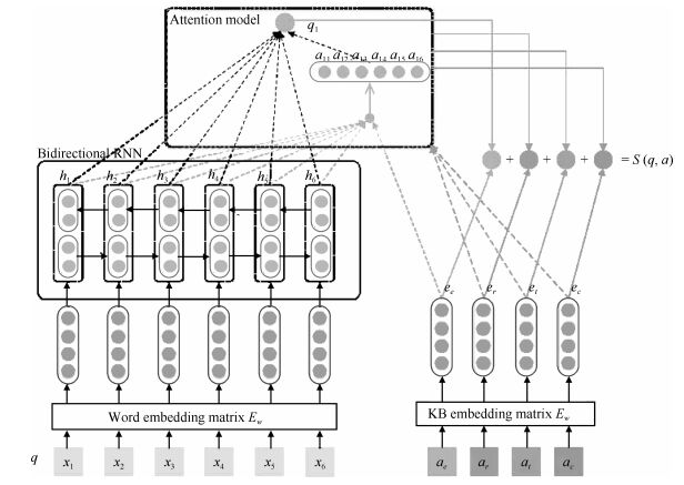
表 Ⅳ THE COMPUTATION TIME OF DIFFERENT METHODS (S)Table Ⅳ THE COMPUTATION TIME OF DIFFERENT METHODS (S)Method Time SNPOM 10.690 EKF 0.40572 EM-EKF 30.766 As a whole, the EM-EKF method is capable of estimating the parameters of the RBF-AR model, and the initial conditions and the noise variances are identified by use of the EM algorithm, which can further improve the modeling precision. Comparison results indicate that the RBF-AR model estimated by the EM-EKF makes more accurate predictions than do the SNPOM and the EKF, although the values of the MSEs using EM-EKF are only slightly smaller than those of the SNPOM and EKF in some cases. However, $F$ test shows there is significant difference between results obtained by the SNPOM and the EM-EKF. Furthermore, the estimation of observation noise variance using EM-EKF is close to the true value, while the estimate of that using SNPOM is unknown, and the observation noise variance in the EKF must be given in advance. Therefore, we can conclude that the EM-EKF method is an advisable choice for estimating RBF-AR model and is especially appropriate for signals disturbed by noise.
5. Conclusion
In this paper, the EM-EKF method is developed to estimate the parameter of RBF-AR model. Firstly, the model is reconstructed as a new type of general radial basis function neural networks. Secondly, to circumvent the EKF's limitation of unknown prior knowledge, the EM is proposed to calculate the initial states and the measurement and process noise variance. By combining the EM and extended Kalman filtering and smoothing process, the EM-EKF method is proposed to estimate the parameters of the RBF-AR model, the initial conditions and the noise variances jointly, and can further improve the modeling precision. Comparisons of the performance of the EM-EKF with the SNPOM and the EKF are performed, and the results indicate that the RBF-AR model estimated by the EM-EKF makes more accurate predictions than do the SNPOM and the EKF, although the EM-EKF is more time-consuming. Moreover, the estimate of observation variance converges to the true value. Finally, F test indicates there is significant difference between results obtained by the SNPOM and the EM-EKF. Our future work would develop the EM-EKF algorithm for RBF-ARX (Peng et al. [2]) estimation and apply the RBF-AR model based on the EM-EKF algorithm to other types of time series and complex systems analysis.
-
表 1 典型英文自动问答系统
Table 1 A list of English QA systems
问答系统 问题类型 数据源 答案形式 相关技术 START What, Who, When等开头的事实型或者定义型问题 START KB、Internet Public Library 一句话或者一段文字 自然语言注释(Natural language annotations)、句子级别的自然语言处理(Sentence-level NLP) AnswerBus 开放领域问答系统 互联网 按照相关程度返回若干个可能的候选答案语句 命名实体抽取(Named entities extraction) Evi 开放领域问答系统 自有结构化知识库(Structured knowledge base), Yelp和第三方网站的数据和API 类似人类语言风格的简明回答 知识表示 AskJeeves 开放领域问答系统 自有问答数据库、互联网 文本、文档链接以及内容摘要 自然语言检索技术(NLP)、人工操作目录索引 Wolfram Alpha 开放领域问答系统 内置的结构化知识库 包含答案信息的各种数据和图表 计算知识引擎(Computational knowledge) Watson 开放领域问答系统 定义了自身的知识框架, 并从海量结构化和半结构化资料中抽取知识构建知识体系 针对用户提问的精准回答 统计机器学习、句法分析、主题分析、信息抽取、知识库集成和知识推理 表 2 典型中文自动问答系统
Table 2 A list of Chinese QA systems
问答系统 问题类型 数据源 答案形式 相关技术 微软小冰 日常聊天伴侣 海量网民聊天语料库 拟人化回答 情感计算、自主知识学习、意图对接对话引擎 京东JIMI 电商售前、售后咨询 自有问答库 文本 深度神经网络、意图识别、命名实体识别 小i机器人 业务咨询 语言知识库以及业务知识库 文本 知识表示、本体理论、分领域的语义网络 度秘 生活服务类咨询 互联网 服务推荐(如餐厅、影院) 全网数据挖掘和聚合 阿里小蜜 导购咨询 自有语料库 文本、语音、网页链接等 知识图谱、语义理解、个性化推荐、深度学习 -
[1] 王飞跃.软件定义的系统与知识自动化:从牛顿到默顿的平行升华.自动化学报, 2013, 41(1): 1-8 http://www.aas.net.cn/CN/abstract/abstract18578.shtmlWang Fei-Yue. Software-defined systems and knowledge automation: a parallel paradigm shift from newton to merton. Acta Automatica Sinica, 2013, 41(1): 1-8 http://www.aas.net.cn/CN/abstract/abstract18578.shtml [2] 王飞跃.机器人的未来发展:从工业自动化到知识自动化.科技导报, 2015, 33(21): 39-44 http://www.cnki.com.cn/Article/CJFDTOTAL-KJDB201521012.htmWang Fei-Yue. On future development of robotics: from industrial automation to knowledge automation. Science & Technology Review, 2015, 33(21): 39-44 http://www.cnki.com.cn/Article/CJFDTOTAL-KJDB201521012.htm [3] Bidian C, Evans M M, Dalkir K. A holistic view of the knowledge life cycle: The Knowledge Management Cycle (KMC) model. Electronic Journal of Knowledge Management, 2014, 12: 85-97 http://www.ejkm.com/issue/download.html?idArticle=563 [4] Simmons R. Answering English questions by computer: a survey. Communications of the ACM, 1965, 8(1): 53-70 doi: 10.1145/363707.363732 [5] Androutsopoulos I, Ritchie G D, Thanisch P. Natural language interfaces to databases—an introduction. Natural Language Engineering, 1995, 1(1): 29-81 http://journals.cambridge.org/action/displayFulltext?type=1&pdftype=1&fid=1313064&volumeId=1&issueId=01&aid=1313056 [6] Indurkhya N, Damerau F J. Handbook of Natural Language Processing (Second Edition). Florida: CRC Press, 2010 [7] 郑实福, 刘挺, 秦兵, 李生.自动问答综述.中文信息学报, 2002, 16(6): 46-52 http://www.cnki.com.cn/Article/CJFDTOTAL-SDKY200704020.htmZheng Shi-Fu, Liu Ting, Qin Bing, Li Sheng. Overview of question-answering. Journal of Chinese Information Processing, 2002, 16(6): 46-52 http://www.cnki.com.cn/Article/CJFDTOTAL-SDKY200704020.htm [8] 汤庸, 林鹭贤, 罗烨敏, 潘炎.基于自动问答系统的信息检索技术研究进展.计算机应用, 2008, 28(11): 2745-2748 http://www.cnki.com.cn/Article/CJFDTOTAL-JSJY200811005.htmTang Yong, Lin Lu-Xian, Luo Ye-Min, Pan Yan. Survey on information retrieval system based on question answering system. Computer Applications, 2008, 28(11): 2745-2748 http://www.cnki.com.cn/Article/CJFDTOTAL-JSJY200811005.htm [9] Bouziane A, Bouchiha D, Doumi N, Malki M. Question answering systems: survey and trends. Procedia Computer Science, 2015, 73: 366-375 doi: 10.1016/j.procs.2015.12.005 [10] Mishra A, Jain S K. A survey on question answering systems with classification. Journal of King Saud University-Computer and Information Sciences, 2016, 28 (3): 345-361 doi: 10.1016/j.jksuci.2014.10.007 [11] Burger J, Cardie C, Chaudhri V, Gaizauskas R, Harabagiu S, Israel D, Jacquemin C, Lin C Y, Maiorano S, Miller G, Moldovan D, Ogden B, Prager J, Riloff E, Singhal A, Shrihari R, Strzalkowski T, Voorhees E M, Weishedel R. Issues, tasks and program structures to roadmap research in question & answering (Q&A). Document Understanding Conferences Roadmapping Documents, 2001. 1-35 [12] 黄昌宁.从IBM深度问答系统战胜顶尖人类选手所想到的.中文信息学报, 2011, 25(6): 21-25 http://www.cnki.com.cn/Article/CJFDTOTAL-MESS201106002.htmHuang Chang-Ning. Thinking about DeepQA beating human champions. Journal of Chinese Information Processing, 2011, 25(6): 21-25 http://www.cnki.com.cn/Article/CJFDTOTAL-MESS201106002.htm [13] 毛先领, 李晓明.问答系统研究综述.计算机科学与探索, 2012, 6(3): 193-207 http://cpfd.cnki.com.cn/Article/CPFDTOTAL-ZGZR200208001041.htmMao Xian-Ling, Li Xiao-Ming. A survey on question and answering systems. Journal of Frontiers of Computer Science and Technology, 2012, 6(3): 193-207 http://cpfd.cnki.com.cn/Article/CPFDTOTAL-ZGZR200208001041.htm [14] 崔桓, 蔡东风, 苗雪雷.基于网络的中文问答系统及信息抽取算法研究.中文信息学报, 2004, 18(3): 24-31 http://www.cnki.com.cn/Article/CJFDTOTAL-MESS200403003.htmCui Huan, Cai Dong-Feng, Miao Xue-Lei. Research on web-based Chinese question answering system and answer extraction. Journal of Chinese Information Processing, 2004, 18(3): 24-31 http://www.cnki.com.cn/Article/CJFDTOTAL-MESS200403003.htm [15] Green B F, Wolf A K, Chomsky C, Laughery K. Baseball, an automatic question-answerer. In: Proceedings of the Western Joint IRE-AIEE-ACM Computer Conference. Los Angeles, California, USA: ACM, 1961. 219-224 [16] Woods W A, Kaplan A M, Nash-Webber B. The lunar sciences natural language information system. Journal of Neuroimmunology, 1972, 174(1-2): 32-38 [17] Hendrix G G, Sacerdoti E D, Sagalowicz D, Slocum J. Developing a natural language interface to complex data. ACM Transactions on Database Systems, 1978, 3(2): 105-147 doi: 10.1145/320251.320253 [18] Warren D H D, Pereira F C N. An efficient easily adaptable system for interpreting natural language queries. Computational Linguistics, 1982, 8(3-4): 110-122 http://dl.acm.org/citation.cfm?id=972944&picked=formats [19] Thompson B H, Thompson F B. Introducing ask, a simple knowledgeable system. In: Proceedings of the 1st Conference on Applied Natural Language Processing. Santa Monica, USA: ACL, 1983. 17-24 [20] Grosz B J, Appelt D E, Martin P A, Pereira F C N. Team: an experiment in the design of transportable natural-language interfaces. Artificial Intelligence, 1987, 32(2): 173-243 doi: 10.1016/0004-3702(87)90011-7 [21] Ott N. Aspects of the automatic generation of SQL statements in a natural language query interface. Information Systems, 1992, 17(2): 147-159 doi: 10.1016/0306-4379(92)90009-C [22] Hindle D. An analogical parser for restricted domains. In: Proceedings of the Workshop on Speech and Natural Language. New York, USA: ACL, 1992. 150-154 [23] Popescu A M, Armanasu A, Etzioni O, Ko D, Yates A. Modern natural language interfaces to databases: composing statistical parsing with semantic tractability. In: Proceedings of the 20th international conference on Computational Linguistics. Geneva, Switzerland: ACL, 2004. Article No.141 [24] Li F, Jagadish H V. Constructing an interactive natural language interface for relational databases. Proceedings of the VLDB Endowment, 2014, 8(1): 73-84 doi: 10.14778/2735461 [25] Llopis M, Ferrández A. How to make a natural language interface to query databases accessible to everyone: an example. Computer Standards and Interfaces, 2013, 35(5): 470-481 doi: 10.1016/j.csi.2012.09.005 [26] Wang S, Meng X F, Liu S. Nchiql: a Chinese natural language query system to databases. In: Proceedings of the 1999 International Symposium on Database Applications in Non-Traditional Environments. Kyoto, Japan: IEEE, 1999. [27] Kupiec J. Murax: a robust linguistic approach for question answering using an on-line encyclopedia. In: Proceedings of the International ACM SIGIR Conference on Research and Development in Information Retrieval. New Orleans, USA: ACM, 2001. 181-190 [28] Katz B. Annotating the World Wide Web using natural language. In: Proceedings of the 5th RIAO Conference on Computer Assisted Information Searching on the Internet. Montreal, Quebec, Canada: ACM, 1997. 136-155 [29] Katz B, Borchardt G C, Felshin S. Natural language annotations for question answering. In: Proceedings of the 19th International Florida Artificial Intelligence Research Society Conference. Florida, USA: AAAI, 2006. 303-306 [30] Burke R D, Hammond K J, Kulyukin V A, Lytinen S L, Tomuro N, Schoenberg S. Question answering from frequently asked question files: experiences with the FAQ finder system. AI Magazine, 1997, 18(2): 57-66 http://www.aaai.org/ojs/index.php/aimagazine/article/view/1294/1195 [31] Hovy E, Gerber L, Hermjakob U, Junk M, Lin C Y. Question answering in webclopedia. In: Proceedings of the TREC-9 Conference. Gaithersburg, USA: NIST, 2000. 655 [32] Ittycheriah A, Franz M, Zhu W J, Ratnaparkhi A, Mammone R J. Ibm's statistical question answering system. Experimental Techniques, 2000, 33(6): 30-37(38) http://citeseerx.ist.psu.edu/viewdoc/download?doi=10.1.1.9.9839&rep=rep1&type=pdf [33] Kwok C, Etzioni O, Weld D S. Scaling question answering to the web. ACM Transactions on Information Systems, 2001, 19(3): 242-262 doi: 10.1145/502115.502117 [34] Dumais S, Banko M, Brill E, Lin J, Ng A. Web question answering: is more always better? In: Proceedings of the 25th Annual International ACM SIGIR Conference on Research and Development in Information Retrieval. Tampere, Finland: ACM, 2002. 291-298 http://dl.acm.org/citation.cfm?id=996350.996430 [35] Khalid M A, Jijkoun V, Rijke M D. The impact of named entity normalization on information retrieval for question answering. In: Proceedings of the 30th European conference on Advances in information retrieval. Berlin, Heidelberg: Springer-Verlag, 2008: 705-710 [36] 刘亚军, 徐易.一种基于加权语义相似度模型的自动问答系统.东南大学学报(自然科学版), 2004, 34(5): 609-612 doi: 10.3969/j.issn.1001-0505.2004.05.011Liu Ya-Jun, Xu Yi. Automatic question answering system based on weighted semantic similarity model. Journal of Southeast University (Natural Science Edition), 2004, 34(5): 609-612 doi: 10.3969/j.issn.1001-0505.2004.05.011 [37] 周法国, 杨炳儒.句子相似度计算新方法及在问答系统中的应用.计算机工程与应用, 2008, 44(1): 165-167 http://www.cnki.com.cn/Article/CJFDTOTAL-JSGG200801052.htmZhou Fa-Guo, Yang Bing-Ru. New method for sentence similarity computing and its application in question answering system. Computer Engineering and Applications, 2008, 44(1): 165-167 http://www.cnki.com.cn/Article/CJFDTOTAL-JSGG200801052.htm [38] Soubbotin M M. Patterns of potential answer expressions as clues to the right answers. In: Proceedings of the 10th Text Retrieval Conference. Gaithersburg, USA: NIST, 2001. 293-302 [39] Lin D K, Pantel P. Discovery of inference rules for question-answering. Natural Language Engineering, 2001, 7(4): 343-360 http://www.patrickpantel.com/download/Papers/2001/jnle01.pdf [40] Mollá D. Learning of graph-based question answering rules. In: Proceedings of the 1st Workshop on Graph Based Methods for Natural Language Processing. New York, USA: ACL, 2006. 37-44 [41] Moldovan D, Clark C, Harabagiu S M, Maiorano S J. Cogex: a logic prover for question answering. In: Proceedings of the 2003 Conference of the North American Chapter of the Association for Computational Linguistics on Human Language Technology. Edmonton, Canada: ACL, 2003. 87-93 [42] Tang L R, Mooney R J. Using multiple clause constructors in inductive logic programming for semantic parsing. In: Proceedings of the European Conference on Machine Learning. Freiburg, Germany: Springer, 2001. 466-477 [43] Zadeh L A. Fuzzy logic = computing with words. IEEE Transactions on Fuzzy Systems, 1996, 4(2): 103-111 doi: 10.1109/91.493904 [44] Clark P, Thompson J, Porter B. A knowledge-based approach to question-answering. In: Proceedings of the 6th National Conference on Artificial Intelligence. Orlando, USA: AAAI, 1999. 43-51 [45] Barker K, Chaudhri V K, Chaw S Y, Clark P E, FAN J, Israel D, Mishra S, Porter B, Romero P, Tecuci D, Yeh P. A question-answering system for AP chemistry. In: Proceedings of the 9th International Conference on Knowledge Representation and Reasoning. Whistler, Canada: AAAI, 2004. 488-497 [46] 刘开瑛.汉语框架语义网构建及其应用技术研究.中文信息学报, 2011, 25(6): 46-53 http://www.cnki.com.cn/Article/CJFDTOTAL-MESS201106006.htmLiu Kai-Ying. Research on Chinese FrameNet construction and application technologies. Journal of Chinese Information Processing, 2011, 25(6): 46-53 http://www.cnki.com.cn/Article/CJFDTOTAL-MESS201106006.htm [47] 王智强, 李茹, 梁吉业, 张旭华, 武娟, 苏娜.基于汉语篇章框架语义分析的阅读理解问答研究.计算机学报, 2016, 38(4): 795-807 doi: 10.11897/SP.J.1016.2016.00795Wang Zhi-Qiang, Li Ru, Liang Ji-Ye, Zhang Xu-Hua, Wu Juan, Su Na. Research on question answering for reading comprehension based on Chinese discourse frame semantic parsing. Chinese Journal of Computers, 2016, 38(4): 795-807 doi: 10.11897/SP.J.1016.2016.00795 [48] Bollacker K, Evans C, Paritosh P, Sturge T, Taylor J. Freebase: a collaboratively created graph database for structuring human knowledge. In: Proceedings of the ACM SIGMOD International Conference on Management of Data. Vancouver, Canada: ACM, 2008. 1247-1250 [49] Suchanek F M, Kasneci G, Weikum G. Yago: a core of semantic knowledge. In: Proceedings of the 16th International Conference on World Wide Web. Banff, Canada: WWW, 2007. 697-706 [50] Hoffart J, Suchanek F M, Berberich K, Weikum G. Yago2: a spatially and temporally enhanced knowledge base from wikipedia. Artificial Intelligence, 2013, 194: 28-61 doi: 10.1016/j.artint.2012.06.001 [51] Yao X C, Van Durme B. Information extraction over structured data: question answering with freebase. In: Proceedings of the 52nd Annual Meeting of the Association for Computational Linguistics. Baltimore, USA: ACL, 2014. 956-966 [52] Yih W T, Chang M W, He X D, Gao J F. Semantic parsing via staged query graph generation: question answering with knowledge base. In: Proceedings of the 53rd Annual Meeting of the Association for Computational Linguistics and the 7th International Joint Conference on Natural Language Processing of the AFNLP. Beijing, China: ACL, 2015.1321-1331 [53] West R, Gabrilovich E, Murphy K, Sun S, Gupta R, Lin D K. Knowledge base completion via search-based question answering. In: Proceedings of the 23rd International Conference on Worldwide Web. Seoul, Korea: ACM, 2014. 515-526 [54] Unger C, Cimiano P. Pythia: compositional meaning construction for ontology-based question answering on the semantic web. In: Proceedings of the Natural Language Processing and Information Systems-International Conference on Applications of Natural Language to Information Systems. Alicante, Spain: Springer, 2011. 153-160 [55] 周永梅, 陶红, 陈姣姣, 张再跃.自动问答系统中的句子相似度算法的研究.计算机技术与发展, 2012, 22(5): 75-78 http://www.cnki.com.cn/Article/CJFDTOTAL-WJFZ201205020.htmZhou Yong-Mei, Tao Hong, Chen Jiao-Jiao, Zhang Zai-Yue. Study on sentence similarity approach of Automatic Ask & Answer System. Computer Technology and Development, 2012, 22(5): 75-78 http://www.cnki.com.cn/Article/CJFDTOTAL-WJFZ201205020.htm [56] 杜文华.本体构建方法比较研究.情报杂志, 2005, 24(10): 24-25 doi: 10.3969/j.issn.1002-1965.2005.10.008Du Wen-Hua. Comparative study of ontology construction methods. Journal of Information, 2005, 24(10): 24-25 doi: 10.3969/j.issn.1002-1965.2005.10.008 [57] 魏顺平, 何克抗.基于文本挖掘的领域本体半自动构建方法研究——以教学设计学科领域本体建设为例.开放教育研究, 2008, 14(5): 95-101 http://www.cnki.com.cn/Article/CJFDTOTAL-JFJJ200805019.htmWei Shun-Ping, He Ke-Kang. Semi-automatic building approach of domain ontology based on text mining——a case study of building instructional design domain ontology. Open Education Research, 2008, 14(5): 95-101 http://www.cnki.com.cn/Article/CJFDTOTAL-JFJJ200805019.htm [58] Iyyer M, Boyd-Graber J, Claudino L, Socher R, Iii H D. A neural network for factoid question answering over paragraphs. In: Proceedings of the Conference on Empirical Methods in Natural Language Processing. Doha, Qatar: ACL, 2014. 633-644 [59] Yih W T, He X D, Meek C. Semantic parsing for single-relation question answering. In: Proceedings of the Meeting of the Association for Computational Linguistics. Baltimore, USA: ACL, 2014. 643-648 [60] Zhang Y Z, Liu K, He S Z, Ji G L, Liu Z Y, Wu H, Zhao J. Question answering over knowledge base with neural attention combining global knowledge information. arXiv: 1606.00979, 2016. [61] Werbos P J. Beyond Regression: new Tools for Prediction and Analysis in the Behavioral Science [Ph.D. dissertation], Harvard University, USA, 1974 [62] Hinton G E, Osindero S, Teh Y W. A fast learning algorithm for deep belief nets. Neural Computation, 2006, 18(7): 1527-1554 doi: 10.1162/neco.2006.18.7.1527 [63] Silver D, Huang A, Maddison C J, Guez A, Sifre L, Van Den Driessche G, Schrittwieser J, Antonoglou I, Panneershelvam V, Lanctot M, Dieleman S, Grewe D, Nham J, Kalchbrenner N, Sutskever I, Lillicrap T, Leach M, Kavukcuoglu K, Graepel T, Hassabis D. Mastering the game of go with deep neural networks and tree search. Nature, 2016, 529(7587): 484-489 doi: 10.1038/nature16961 [64] 刘康, 张元哲, 纪国良, 来斯惟, 赵军.基于表示学习的知识库问答研究进展与展望.自动化学报, 2016, 42(6): 807-818 http://www.aas.net.cn/CN/abstract/abstract18872.shtmlLiu Kang, Zhang Yuan-Zhe, Ji Guo-Liang, Lai Si-Wei, Zhao Jun. Representation learning for question answering over knowledge base: an overview. Acta Automatica Sinica, 2016, 42(6): 807-818 http://www.aas.net.cn/CN/abstract/abstract18872.shtml [65] Zheng Z P. AnswerBus question answering system. In: Proceedings of the 2nd International Conference on Human Language Technology Research. San Diego, USA: ACM, 2002. 399-404 [66] Tunstall-Pedoe W. True knowledge: open-domain question answering using structured knowledge and inference. AI Magazine, 2010, 31(3): 80-92 doi: 10.1609/aimag.v31i3.2298 [67] Hajishirzi H, Mueller E T. Question answering in natural language narratives using symbolic probabilistic reasoning. In: Proceedings of the 25th International Florida Articial Intelligence Research Society Conference. Marco Island, USA: AAAI, 2012. 38-43 [68] Lally A, Prager J M, McCord M C, Boguraev B K, Patwardhan S, Fan J, FODOR P, Chu-Ca J. Question analysis: how watson reads a clue. IBM Journal of Research and Development, 2012, 56(3-4): 2:1-2:14 http://ieeexplore.ieee.org/xpl/articleDetails.jsp?reload=true&tp=&arnumber=6177727 [69] Kalyanpur A, Patwardhan S, Boguraev B K, Lally A, Chu-Carroll J. Fact-based question decomposition in DeePQA. IBM Journal of Research and Development, 2012, 56(3): 388-389 http://ieeexplore.ieee.org/xpl/abstractKeywords.jsp?reload=true&arnumber=6177726&filter%3DAND%28p_IS_Number%3A6177717%29 [70] Gondek D C, Lally A, Kalyanpur A, Murdock J W, Duboue P A, Zhang L, Pan Y, Qiu Z M. A framework for merging and ranking of answers in DeePQA. IBM Journal of Research and Development, 2012, 56(3-4): 14:1-14:12 http://ieeexplore.ieee.org/xpl/articleDetails.jsp?arnumber=6177810& [71] Dang H T, Kelly D, Lin J J. Overview of the TREC 2007 question answering track. In: Proceedings of the 16th Text Retrieval Conference. Gaithersburg, USA: NIST, 2007. 115-123 [72] Olvera-Lobo M D, Gutiérrez-Artacho J. Question answering track evaluation in TREC, CLEF and NTCIR. Advances in Intelligent Systems and Computing, 2015, 353: 13-22 doi: 10.1007/978-3-319-16486-1 [73] Peñas A, Forner P, Sutcliffe R, Rodrigo Á, Forăscu C, Alegria I, Giampiccolo D, Moreau N, Osenova P. Overview of ResPubliQA 2009: question answering evaluation over European legislation. In: Proceedings of the 10th Cross-Language Evaluation Forum Conference on Multilingual Information Access Evaluation: text Retrieval Experiments. Corfu, Greece: Springer, 2010. 174-196 [74] Agichtein E, Carmel D, Harman D, Pelleg D, Pinter Y. Overview of the TREC 2015 LiveQA track. In: Proceedings of the 24th TextREtrieval Conference. Gaithersburg, USA: NIST, 2015. 1-9 -