2.845

2023影响因子

(CJCR)

  • 中文核心
  • EI
  • 中国科技核心
  • Scopus
  • CSCD
  • 英国科学文摘

留言板

尊敬的读者、作者、审稿人, 关于本刊的投稿、审稿、编辑和出版的任何问题, 您可以本页添加留言。我们将尽快给您答复。谢谢您的支持!

姓名
邮箱
手机号码
标题
留言内容
验证码

非完整性约束的平面多智能体位置时变一致性控制

赵俊 刘国平

侯利民, 王龙洋, 王怀震. 基于NDOB的匹配/非匹配不确定性系统滑模控制. 自动化学报, 2017, 43(7): 1257-1264. doi: 10.16383/j.aas.2017.e160014
引用本文: 赵俊, 刘国平. 非完整性约束的平面多智能体位置时变一致性控制. 自动化学报, 2017, 43(7): 1169-1177. doi: 10.16383/j.aas.2017.c160591
Hou Limin, Wang Longyang, Wang Huaizhen. SMC for Systems With Matched and Mismatched Uncertainties and Disturbances Based on NDOB. ACTA AUTOMATICA SINICA, 2017, 43(7): 1257-1264. doi: 10.16383/j.aas.2017.e160014
Citation: ZHAO Jun, LIU Guo-Ping. Position Time-varying Consensus Control for Multiple Planar Agents with Non-holonomic Constraint. ACTA AUTOMATICA SINICA, 2017, 43(7): 1169-1177. doi: 10.16383/j.aas.2017.c160591

非完整性约束的平面多智能体位置时变一致性控制

doi: 10.16383/j.aas.2017.c160591
基金项目: 

国家自然科学基金 61690212

国家自然科学基金 61333003

详细信息
    作者简介:

    刘国平 哈尔滨工业大学教授, IEEE Fellow.主要研究方向包括网络化控制系统, 多智能体控制, 非线性系统辨识与控制, 多目标最优控制.E-mail:gpliu@hit.edu.cn

    通讯作者:

    赵俊 哈尔滨工业大学航天学院博士生.2011年获得西南科技大学硕士学位.主要研究方向为网络化控制系统, 多智能体时变编队控制.本文通信作者. E-mail:zjlzl1031@icloud.com

Position Time-varying Consensus Control for Multiple Planar Agents with Non-holonomic Constraint

Funds: 

National Natural Science Foundation of China 61690212

National Natural Science Foundation of China 61333003

More Information
    Author Bio:

      Professor at the Harbin Institute of Techonology, IEEE Fellow. His research interest covers networked control systems, multi-agent systems, identify and control of non-liner systems, and multi-object optimization

    Corresponding author: ZHAO Jun  Ph. D. candidates at the School of Astronautics, Harbin Instititue of Technology. He received his master degree from South West University of Science and Technology in 2011. His research interest covers formation control of networked control systems and time-variant formation of multi-agnet systems. Corresponding author of this paper. E-mail:zjlzl1031@icloud.com
  • 摘要: 多智能体的通用一致性协议被广泛用于智能体的编队控制问题中.在实际工程中,多智能体系统为了完成期望的协作控制,智能体之间的位置关系通常是时变的.目前,在多智能体编队控制问题中,尽管已有研究成果能够解决多智能体某些特殊类型的时变编队控制,但对一般性的时变编队还没有成熟的研究成果.本文以受非完整性约束的平面多智能体为研究对象,提出了平面非完整性多智能体的位置时变一致性协议.实验结果表明:本文提出的位置时变一致性协议能够有效解决平面非完整性多智能体系统一般性的时变编队问题.
  • In recent years, the control methods for systems affected by uncertainties and disturbances have been focused by researchers [1]-[7]. Compared to other control methods, sliding mode control (SMC) has attracted a significant interest due to its conceptual simplicity, easy implementation, and robustness to external disturbances and model uncertainties [8]-[10]. SMC is a nonlinear control strategy that forces the closed loop trajectories to the switching manifold in finite-time using a discontinuous feedback control action. Therefore, SMC has been widely used in many applications, such as motion control, process control, etc. However, the conventional sliding mode control has a violent chattering phenomenon in the process, which can degrade the system performance. Moreover, it can guarantee invariance only if the uncertainties and disturbances satisfy the matching conditions, and cannot attenuate mismatched uncertainties and disturbances effectively.

    Note that the matched and mismatched uncertainties and disturbances widely exist in practical engineering, such as power systems [11], electronic systems [12], [13] and motor systems [14]. The sliding motion of the traditional SMC is severely affected by the mismatched uncertainties and disturbances, and the well-known robustness of SMC does not hold any more. Algorithms like LMI-based control [15], [16], adaptive control [17], [18], back stepping based control [19], and integral sliding-mode control [20], [21] are proposed to handle mismatched uncertainties in a robust way, but the price is that the nominal control performance is compromised.

    As a practical alternative approach, disturbance observer-based control has been proven to be promising and effective in compensating the effects of unknown external disturbances and model uncertainties in control systems as well as it will not deteriorate the existing controller [22], [23]. It could completely remove the non-vanishing disturbances from system as long as they can be estimated accurately [24]. Recently, several authors introduced a disturbance observer (DOB) for SMC to alleviate the chattering problem and retain its nominal control performance [25]-[29]. The idea is to construct the control law by combining the SMC feedback with the disturbance estimation based-feed forward compensation straightforwardly. However, these methods given in [25]-[29] are only available for the matched uncertain systems. A nonlinear extension of DO has been proposed by W. H. Chen, which estimates matched as well as mismatched disturbances [30], [31]. Reference [1] extends a recent result on sliding mode control for general nth order systems with a larger class of mismatched uncertainties by proposing an extended disturbance observer. Reference [13] investigates an extended state observer (ESO)-based sliding mode control (SMC) approach for pulse width modulation-based DC-DC buck converter systems subject to mismatched disturbances, the proposed method obtains a better disturbance rejection ability even the disturbances do not satisfy the so-called matching condition. A novel sliding-mode control based on the disturbance estimation by a nonlinear disturbance observer (NDOB) based SMC in [14] is only proposed to deal with mismatched uncertainties, it can ensure the system performance and reduce the chattering.

    In this paper, aiming to improve the performance of the system affected by mismatched/matched uncertainties and disturbances, a novel nonlinear control scheme is proposed, where the SMC scheme is integrated with NDOB. By fully taking into account the estimation value of disturbances, a new sliding-mode surface is firstly designed which is insensitive to not only matched disturbances but also mismatched ones. In this paper, the contributions are listed as follows:

    1) The control is proposed for a general system of $n$ order, having mismatched/matched uncertainties and disturbances.

    2) The novel sliding surface is extended for a general system of n order and modified to enable improvement in the performance of the system without causing a large increase in the control.

    3) The proposed method exhibits the properties of nominal performance recovery and chattering reduction as well as excellent dynamic and static performance as compared with the traditional SMC.

    The paper is organized as follows: the problem of nominal sliding mode controller design with mismatched and matched uncertainties and disturbances for a class of nonlinear system is stated in Section 2. Generalization of NDOB, novel sliding surface design and the stability analysis are derived in Section 3. The simulation results are presented in Section 4, followed by some concluding remarks in Section 5.

    Consider a class of single-input single-output dynamic systems with matched and mismatched uncertainties, depicted by

    $ \begin{equation} \left\{\begin{array}{llllll} & \!\!\!\!\!\!\!{{\dot x}_i} ={x_{i + 1}} + {d_i}(t)\\ & ~\vdots\\ & \!\!\!\!\!\!\!{{\dot x}_n} =a(x) + b(x)u + {d_n}(t)\\ & \!\!\!\!\!\!\!y ={x_1} \end{array} \right. \ i= 1, \ldots, n - 1\ \end{equation} $

    (1)

    where $x = {\left[{{x_1} \ldots {x_n}} \right]^T}$ is the state vector, $u$ is the control input, $y$ is the controlled output, ${d_i}(t)$ and ${d_n}(t)$ are the mismatched and matched uncertainties and disturbances, respectively. $a(x)$ and $b(x)$ denote smooth nominal functions.

    Taking a second-order system as an illustration, we can get the control model of the system:

    $ \begin{equation} \left\{ \begin{array}{lllll} & \!\!\!\!\!\!\!{{\dot x}_1} ={x_2} + {d_1}(t)\\ & \!\!\!\!\!\!\!{{\dot x}_2} = a(x) + b(x)u + {d_2}(t)\\ & \!\!\!\!\!\!\!y ={x_1} \end{array} \right.. \end{equation} $

    (2)

    Assumption 1: The lumped disturbances ${d_1}(t)$ , ${d_2}(t)$ in (2) are bounded and defined by .

    The sliding mode surface and control law of the traditional SMC is usually designed as follows:

    $ \begin{equation} {s_1} = {x_2} + {k_1}{x_1} \end{equation} $

    (3)

    $ \begin{equation} u = - {b^{ - 1}}(x)\left[{{k_1}{x_2} + {\eta _1}{\rm sgn}(s_1) + a(x)} \right] \end{equation} $

    (4)

    where ${k_1} > 0$ is a design constant, ${\eta _1} > 0$ is the switching gain to be designed. Taking the derivative of (3), and combining (2) and (4) gives

    $ \begin{equation} {\dot s_1} = - {\eta _1}{\rm sgn}(s_1) + {k_1}{d_1}(t) + {d_2}(t). \end{equation} $

    (5)

    The states of (2) will reach the sliding mode surface ${s_1} = 0$ in finite time if the switching gain ${\eta _1}$ in the control law (4) is devised such that ${\eta _1} > {d^*}$ . Once the nominal sliding surface ${s_1} = 0$ is reached, the sliding motion is obtained and given by

    $ \begin{equation} {\dot x_1} + {k_1}{x_1} = {d_1}(t). \end{equation} $

    (6)

    Remark 1: Equation (6) implies that if the ${d_1}(t) = 0$ , the system states can be driven to the desired equilibrium point, which implies that the conventional SMC is insensitive to matched disturbance. However, in the existence of mismatched disturbance ${d_1}(t) \ne 0$ , the system state ${x_1}$ is affected by the mismatched disturbance and does not converge to zero in finite time although the control law can force the system states to reach the sliding-mode surface in a finite time. To this end, it is an essential reason why the nominal SMC design is only insensitive to matched disturbance but sensitive to mismatched disturbance.

    In this paper, the matched and mismatched disturbance rejection problem is considered for (1). A novel sliding mode controller based on NDOB is proposed by the following two steps. First, an NDOB is employed to estimate the matched and mismatched disturbances. A novel sliding mode controller is then designed for the system based on the disturbance observation. The control structure of the second-order system is designed as Fig. 1.

    图 1  Control structure of second-order system.
    Fig. 1  Control structure of second-order system.

    A nonlinear disturbance observer (NDOB), which is adopted to estimate the disturbance in [14]. Consider a class of nonlinear systems with uncertainties and external disturbance:

    $ \begin{equation} \left\{ \begin{array}{ccccc} \dot x =f(x) + {g_1}(x)u + {g_2}(x)d(t)\\ y =h(x)~~~~~~~~~~~~~~~~~~~~~~~~~~ \end{array} \right.. \end{equation} $

    (7)

    A NDOB is used to estimate the compound disturbance of the system and compensate accordingly, in order to improve the robustness of the controller. The NDOB is introduced and depicted by

    $ \begin{equation} \left\{ \begin{array}{lllllll} & \!\!\!\!\!\!\!\dot z = - l{g_2}(x)z - l\left[{{g_2}(x)lx + f(x) + {g_1}(x)u} \right]\\ & \!\!\!\!\!\!\!\hat d(t) = z + lx \end{array} \right. \end{equation} $

    (8)

    where $\hat d(t)$ is the estimation vector of the disturbance vector $d(t)$ , and $z$ is the internal state vector of the nonlinear observer. $l$ is the disturbance observer gain matrix to be designed.

    Assumption 2: The derivative of the disturbance in system (1) is bounded and satisfies

    $ \begin{equation*}\mathop {\lim }\limits_{t \to \infty } d_i^{(j)}(t) = 0, \quad \quad i = 1, \ldots, n; j = 1, \ldots, n - 1.\end{equation*} $

    Remark 2: This assumption satisfies the requirements of the simulation sample. An extended disturbance observer is proposed in [1], which can observe a class of systems with mismatched uncertainties and get for the sliding mode surface and $u$ . A nonlinear disturbance observer is designed to observe and get for the sliding mode surface and $u$ in our paper.

    The disturbance estimation error of the NDOB is defined:

    $ \begin{equation} {e_d}(t) = d(t) - \hat d(t). \end{equation} $

    (9)

    The error dynamics can be derived as

    $ \begin{align} & {{{\dot{e}}}_{d}}(t)=\dot{d}(t)-\dot{\hat{d}}(t) \\ & \ \ \ \ \ \ \ \ \ =\dot{d}(t)-\dot{z}-l\left[f(x)+{{g}_{1}}(x)u+{{g}_{2}}(x)d(t) \right]. \\ \end{align} $

    (10)

    Substituting the value of $\dot z$ , error dynamics reduce to

    $ \begin{equation} {\dot e_d}(t) = \dot d(t) - {lg_2}(x){e_d}(t). \end{equation} $

    (11)

    Lemma 1 [7]: Suppose that Assumptions 1 and 2 are satisfied for (7). The disturbance estimation $\hat d(t)$ of NDOB (8) can track the disturbance $d$ of (7) asymptotically as long as the observer gain $l$ is chosen such that $lg_2(x) > 0$ holds, which implies that ${\dot e_d}(t) + {lg_2}(x){e_d}(t) = 0$ , the estimation error will converge to zero asymptotically.

    Consider the system

    $ \begin{equation} \dot x = f(t, x, u) \end{equation} $

    (12)

    where is piecewise continuous in $t$ and locally Lipschitz in $x$ and $u$ . The input $u(t)$ is a piecewise continuous, bounded function of $t$ for all $t \ge {0}$ .

    Definition 1: The system (12) is said to be input-to-state stable (ISS) if there exist a class $\kappa \iota $ function and a class $\kappa$ function $\gamma $ such that for any initial state $x({t_0})$ and any bounded input $u(t)$ , the solution $x(t)$ exists for all $t \ge {t_0}$ and satisfies

    $ \begin{equation} \left\| {x(t)} \right\| \le \beta (\left\| {x({t_0})} \right\|, t- {t_0}) + \gamma (\mathop {\sup }\limits_{{t_0} \le \tau \le t} \left\| {u(\tau )} \right\|). \end{equation} $

    (13)

    Such a function $\gamma$ in (13) is referred to as an ISS-gain for (12). ISS implies that (12) is bounded-input bounded-state stable when $u \ne 0$ and its zero solution (with $u = 0$ ) is globally asymptotically stable.

    Lemma 2 [14]: Consider a nonlinear system $\dot x = F(x, w)$ , which is input-to-state stable (ISS). If the input satisfies $\mathop {\lim }_{t \to \infty } w(t) = 0$ , then the state .

    A novel sliding mode manifold for (2) under matched and mismatched disturbances is designed as

    $ \begin{equation} {s_2} = {x_2} + {k_2}{x_1} + {\hat d_1}(t). \end{equation} $

    (14)

    Theorem 1: Considering the above (2) with matched and mismatched disturbances, we proposed sliding-mode surface (14), if the control law is designed as follows:

    $ \begin{align} u = & - {b^{ - 1}}(x)\Big\{ {k_2}\left[{{x_2} + {{\hat d}_1}(t)} \right] + {\eta _2}{\rm sgn}({s_2})\nonumber\\ & + a(x) + {{\hat d}_2}(t) + {{\dot {\hat d}_1}}(t) \Big\}. \end{align} $

    (15)

    Suppose the second-order system satisfies Assumptions 1 and 2, the observer gain $l$ is chosen such that ${\lg}{_2}(x) > 0$ holds, if the switching gain is chosen such that and ${k_2} > 0$ , then the closed-loop system is asymptotically stable.

    Proof: Consider a candidate Lyapunov function as

    $ \begin{equation} {V_1} = \frac{1}{2}s_2^T{s_2}. \end{equation} $

    (16)

    Taking derivative of $V$ in (16), we obtain that

    $ \begin{equation} {\dot V_1} = {s_2}{\dot s_2} = {s_2}({\dot x_2} + {k_2}{\dot x_1} + \dot{\hat{d}}_1 (t). \end{equation} $

    (17)

    Substituting (15) into (2) yields

    $ \begin{align} {{\dot x}_2} = & a(x) + b(x)u + {d_2}(t)\nonumber\\ = & a(x) - b(x) \times {b^{ - 1}}(x)\Big\{ {k_2}\left[{{x_2} + {{\hat d}_1}(t)} \right] + {\eta _2}{\rm sgn}({s_2})\nonumber\\ & + a(x) + {{\hat d}_2}(t) + {{\dot {\hat d}_1}(t)}\Big\} + {d_2}(t). \end{align} $

    (18)

    Substituting (18) into (17) yields

    $ \begin{align} {\dot V}_1= & {s_2} \Big\{ - {k_2}\left[{{x_2} + {{\hat d}_1}(t)} \right] - {\eta _2}{\rm sgn}(s) - {{\hat d}_2}(t)\nonumber\\ & - {{\dot {\hat d}_1}(t)} + {d_2}(t) + {k_2}{x_2} + {k_2}{d_1}(t) + {{\dot {\hat d}_1}(t)} \Big\}\nonumber\\[1mm] = & {s_2} \Big\{ - {k_2}{{\hat d}_1}(t) - {\eta _2}{\rm sgn}(s) - {{\hat d}_2}(t) + {d_2}(t) + {k_2}{d_1}(t) \Big\}\nonumber\\ = & {s_2}\left( { - {\eta _2}{\rm sgn}({s_2}) + {k_2}{e_{d1}} + {e_{d2}}} \right)\nonumber\\[1mm] \le & \left[{-{\eta _2} + {k_2}{e_{d1}} + {e_{d2}}} \right]\left| {{s_2}} \right|\nonumber\\[1mm] = & - \sqrt 2 \left[{{\eta _2}-({k_2}{e_{d1}} + {e_{d2}})} \right]V_1^{\frac{1}{2}} \end{align} $

    (19)

    where ${e_{d1}} = {d_1} - {\hat d_1}$ , .

    It can be derived from (19) that the system states will reach the defined sliding surface ${s_2} = 0$ in finite time when . The condition implies

    $ \begin{equation} {\dot x_1} = - {k_2}{x_1} + {e_{d1}}. \end{equation} $

    (20)

    With this result, it can be derived that (20) is ISS. According to Lemma 2, we know that the system states satisfy and . This implies that the system states can converge to the desired equilibrium point along the sliding surface asymptotically under the proposed control law.

    Remark 3: Since the matched and mismatched disturbances have been precisely estimated by the NDOB, the switching gain of the proposed method can be designed much smaller than those of the traditional SMC, because the magnitude of the estimation error ${e_d}$ is much smaller than the magnitude of the disturbance $d$ . The chattering problem can be alleviated to some extent in the case the nominal performance of the sliding mode control is retained.

    Consider the following third-order system, depicted by

    $ \begin{equation} \left\{ \begin{array}{llll} {{\dot x}_1} = {x_2} + {d_1}(t)\\ {{\dot x}_2} = {x_3} + {d_2}(t)\\ {{\dot x}_3} = a(x) + b(x)u + {d_3}(t)\\ y = {x_1}. \end{array} \right. \end{equation} $

    (21)

    A sliding mode manifold for (21) is designed as

    $ \begin{equation} {s_3} = {x_3} + {x_2} + {k_3}{x_1} + {\hat d_1}(t) + {\hat d_2}(t) + \dot{\hat{d}}_1(t). \end{equation} $

    (22)

    Theorem 2: Considering the above (21) with matched and mismatched disturbances, we proposed sliding-mode surface (22), if the control law is designed as follows:

    $ \begin{align} u= & - {b^{ - 1}}(x)\Big\{ {k_3}\left[{{x_2}+ {{\hat d}_1}(t)} \right] + {\eta _3}{\rm sgn}({s_3}) + {x_3} + a(x)\nonumber\\ & + {{\hat d}_2}(t)+ {{\hat d}_3}(t) + {{\dot {\hat d}_1}(t)}+{{\dot {\hat d}_2}(t)}+{{\ddot {\hat d}_1}(t)} \Big\}. \end{align} $

    (23)

    Suppose the third-order system satisfies Assumptions 1 and 2, the observer gain $l$ is chosen such that ${\lg}{_2}(x) > 0$ holds, if the switching gain is chosen such that ${k_3} > 0$ and , then the closed-loop system is asymptotically stable.

    A sliding mode manifold for (1) in the case $n > 2$ is designed as

    $\begin{equation} {s_n} = \sum\limits_{i = 2}^n {{x_i}} + {k_n}{x_1} + \sum\limits_{j = 1}^{n - 1} {\sum\limits_{i = 1}^{n - j} {\hat d_i^{(j - 1)}(t)} }. \end{equation} $

    (24)

    Theorem 3: Considering the above system (1) with matched and mismatched disturbances, we proposed sliding-mode surface (24), if the control law is designed as follows:

    $ \begin{align} u = & - {b^{ - 1}}(x)\Big\{ {k_n}\left[{{x_2} + {{\hat d}_1}(t)} \right] + {\eta _n}{\rm sgn}({s_n}) + \sum\limits_{i = 3}^n {{x_i}} \nonumber\\ & + a(x) + \sum\limits_{i = 2}^n {{{\hat d}_i}(t)} + \sum\limits_{j = 1}^{n - 1} {\sum\limits_{i = 1}^{n - j} {\hat d_i^{(j)}(t)} } \Big\}. \end{align} $

    (25)

    Suppose the general high-order system satisfies Assumptions 1 and 2, the observer gain $l$ is chosen such that ${\lg}{_2}(x)> 0$ holds, if the switching gain is chosen such that and ${k_n} > 0$ , then the closed-loop system is asymptotically stable.

    Proof: Consider a candidate Lyapunov function as

    $ \begin{equation} {V_n} = \frac{1}{2}s_n^T{s_n}. \end{equation} $

    (26)

    Taking derivative of $V$ in (26), we obtain that

    $ \begin{align} {{\dot V}_n} = & {s_n}{{\dot s}_n} = {s_n}\big(\sum\limits_{i = 2}^n {{{\dot x}_i}} + {k_n}{{\dot x}_1} + \sum\limits_{j = 1}^{n - 1} {\sum\limits_{i = 1}^{n - j} {\hat d_i^{(j)}(t)} } \big) \nonumber\\ = & {s_n}\Big[ {x_3} + {d_2} + {x_4} + {d_3} + \cdots + {x_n} + {d_{n-1}} + a(x)\nonumber\\ & + b(x)u + {d_n}(t) + {k_n}{x_2} + {k_n}{d_1} + \sum\limits_{j = 1}^{n-1} {\sum\limits_{i = 1}^{n-j} {\hat d_i^{(j)}(t)} } \Big]. \end{align} $

    (27)

    Substituting (25) into (27) yields

    $\begin{align}{{\dot V}_n}= & {s_n}\Bigg\{ {x_3} + {d_2} + {x_4} + {d_3} + \cdots + {x_n} + {d_{n - 1}} + a(x)\nonumber\\ & - b(x)\!\! \times\!\! {b^{ - 1}}(x)\bigg\{ {k_n}\left[{{x_2} + {{\hat d}_1}(t)} \right] + {\eta _n}{\rm sgn}({s_n})\nonumber\\ & + \sum\limits_{i = 3}^n {{x_i}} + a(x) + \sum\limits_{i = 2}^n {{{\hat d}_i}(t)} + \sum\limits_{j = 1}^{n - 1} {\sum\limits_{i = 1}^{n - j} {\hat d_i^{(j)}(t)} } \bigg\}\nonumber\\ & + {d_n}(t) + {k_n}{x_2} + {k_n}{d_1} + \sum\limits_{j = 1}^{n - 1} {\sum\limits_{i = 1}^{n - j} {\hat d_i^{(j)}(t)} } \Bigg\}\nonumber\\ = & {s_n}\Bigg[{-{\eta _n}{\rm sgn}({s_n}) + {k_n}{e_{d1}} + \sum\limits_{i = 2}^n {{e_{di}}} } \Bigg]\nonumber\\ \le & \left| {{s_n}} \right|( - {\eta _n} + {k_n}{e_{d1}} + \sum\limits_{i = 2}^n {{e_{di}}}). \end{align} $

    (28)

    It can be derived from ${\dot V_n}$ (28) that the system states will reach the defined sliding surface ${s_n} = 0$ in finite time when . The condition ${s_n} = 0$ implies:

    $ \begin{equation} x_1^{(n - 1)} + x_1^{(n - 2)} + \ldots + {\dot x_1} + {k_n}{x_1} - \sum\limits_{j = 1}^{n - 1} {\sum\limits_{i = 1}^{n - j} {e_{di}^{(j - 1)}}} = 0. \end{equation} $

    (29)

    We can define

    $ \begin{equation} \left\{ {\begin{array}{*{20}{lll}} {{Y_1} = {x_1}}\\ {{Y_2} = {{\dot x}_1}}\\ ~~~~\vdots \\ {{Y_{n - 1}} = x_1^{(n - 2)}} \end{array}} \right.. \end{equation} $

    (30)

    Equation (29) is given by

    $ \begin{equation} \dot Y\! =\! \left[\! {\begin{array}{*{20}{c}} 0 & 1 & 0 & \cdots & 0\\ 0 & 0 & 1 & 0 & 0\\ \vdots & \vdots & \ddots & \vdots & \\ 0 & 0 & \cdots & 0 & 1\\ {-{k_n}} & {-1} & {-1} & \cdots & { - 1} \end{array}} \right]Y + \left[{\begin{array}{*{20}{c}} 0\\ 0\\ \vdots \\ 0\\ {\sum\limits_{j = 1}^{n-1} {\sum\limits_{i = 1}^{n-j} {e_{di}^{(j-1)}} } } \end{array}} \right]. \end{equation} $

    (31)

    Equation (31) can also be expressed as

    $ \begin{equation} \dot Y = AY + B\sum\limits_{j = 1}^{n - 1} {\sum\limits_{i = 1}^{n - j} {e_{di}^{(j - 1)}} } \end{equation} $

    (32)

    where ,

    In view of Assumption 1 and (11), we can conclude:

    $ \begin{equation} \begin{array}{llllllll} \sum\limits_{j = 1}^{n - 1} {\sum\limits_{i = 1}^{n - j} {e_{di}^{(j - 1)}} } = \sum\limits_{i = 1}^{n - 1} {{e_{di}}} + \sum\limits_{i = 1}^{n - 2} {({{\dot d}_i} - {{\lg}_2}{e_{di}})} \\+ \sum\limits_{i = 1}^{n - 3} {({{\ddot d}_i} - {{\lg}_2}{{\dot d}_i} + {l^2}g_2^2{e_{di}})} + \cdots \\+ \sum\limits_{i = 1}^2 {(d_i^{n - 3} - {{\rm lg}_2}d_i^{n - 4} + {l^2}g_2^2d_i^{n - 5} - \cdots - {l^{n - 3}}g_2^{n - 3}{e_{di}})} \\ + (d_1^{n - 2} - {{\rm lg}_2}d_1^{n - 3} + {l^2}g_2^2d_1^{n - 4} - \cdots - {l^{n - 2}}g_2^{n - 2}{e_{d1}}). \end{array} \end{equation} $

    (33)

    Combining Lemma 1, (11) and (33) can get:

    $ \begin{equation} \mathop {\lim }\limits_{t \to \infty } \sum\limits_{j = 1}^{n - 1} {\sum\limits_{i = 1}^{n - j} {e_{di}^{(j - 1)}} } = 0. \end{equation} $

    (34)

    According to the principle of Hurwitz matrix, it can be designed $A$ as a Hurwitz matrix by selecting a proper ${k_n}$ . Taking as an input of (32), it follows from Lemma 2 that (32) is ISS. It is derived from the definition of ISS that the state of (32) converges to zero as $t \to \infty $ , that is, . This implies that the system states can converge to zero along the sliding surface asymptotically under the proposed control law.

    Remark 4: The above proof implies that states of system can be driven to the desired equilibrium point and the control law can force the system states to reach the sliding-mode surface in finite time. This is the main reason why the proposed NDOB-based SMC method is insensitive to matched uncertainties and disturbances as well as mismatched uncertainties and disturbances.

    To evaluate the effectiveness of the proposed method, two examples are given below.

    $ \begin{equation} \left\{ \begin{array}{l} {{\dot x}_1} = {x_2} + {d_1}(t)\\ {{\dot x}_2} = {x_3} + {d_2}(t)\\ {{\dot x}_3} = - 2{x_2} - {x_3} + {e^{{x_1}}} + u + {d_3}(t)\\ y = {x_1}. \end{array} \right. \end{equation} $

    (35)

    In order to show the advantages of the NDOB-based SMC method proposed in this paper compared with the nominal sliding control, we will use simulations to compare the performance between them for (35). The control parameters of the two control methods are listed in Table Ⅰ. Consider the initial states of (35) as . Mismatched/matched uncertainties and disturbances ${d_1} = 1.5, {d_2} = 0.5, {d_3} = 1$ are imposed on the system at 25, 30, 15 sec respectively. The simulation results are shown in Figs. 2-4.

    表 Ⅰ  Control Parameters for the Numerical Example in Case 1
    Table Ⅰ  Control Parameters for the Numerical Example in Case 1
    Controllers Parameters
    SMC1 k = 8, η= 16
    SMC2 k = 8, η= 10
    NDOB-SMC k = 8, η = 10, l = diag{6, 6, 6}
    下载: 导出CSV 
    | 显示表格
    图 2  System state variables.
    Fig. 2  System state variables.
    图 3  Control signal of system.
    Fig. 3  Control signal of system.
    图 4  Reference/estimation uncertainties and disturbances.
    Fig. 4  Reference/estimation uncertainties and disturbances.

    The reference/estimation uncertainties and disturbances of the system are shown in Fig. 4. It can be seen from Fig. 4 that the proposed control gives a better estimation of the disturbance and a better performance.

    In $d-q$ coordinates the permanent magnet synchronous motor (PMSM) dynamic equation can be written as

    $ \begin{equation} \dot \omega = - a\omega + b{i_q} - d \end{equation} $

    (36)

    where $a = B/J$ , $b = 3p{\psi _f}/{(2J)}$ , $d = T_L/J$ . $\omega$ is the rotor angular velocity, $p$ is the number of pole pairs, ${\psi _f}$ is the flux linkage, ${T_L}$ is the load torque, $B$ is the viscous friction coefficient, $J$ is the moment of inertia.

    The state variable of speed error is defined as and its derivative as follows:

    $ \begin{equation} {\dot x_1} = {x_2} = {\dot \omega _{\rm ref}} - \dot \omega = {\dot \omega _{\rm ref}} + a\omega - b{i_q} + d \end{equation} $

    (37)

    where ${\omega _{\rm ref}}$ is the reference speed signal.

    The speed error derivative dynamic equation of the motor can be expressed as follows, with the parameters variations taken into account:

    $ \begin{eqnarray} {{\dot x}_1} & = & {{\dot \omega }_{\rm ref}} + a\omega + \Delta a\omega - b{i_q} - \Delta b{i_q} + d + \Delta d\nonumber\\ & = & {x_2} + \Delta a\omega - \Delta b{i_q} + \Delta d\nonumber\\ & = & {x_2} + {d_1} \end{eqnarray} $

    (38)

    where $\Delta a$ , $\Delta b$ , and $\Delta d$ are parameter variations of $a$ , $b$ , $d$ , and is considered as mismatched uncertainties.

    The second-order model of speed error derivative dynamic equation of PMSM system is described by

    $ \begin{equation} {\dot x_2} = {\ddot \omega _{\rm ref}} - \ddot \omega = {\ddot \omega _{\rm ref}} + a\dot \omega - b{\dot i_q} + \dot d. \end{equation} $

    (39)

    ${\dot x_2}$ can be expressed as follows, with the parameters variations taken into account:

    $ \begin{eqnarray} {{\dot x}_2} & = & {{\ddot \omega }_{\rm ref}} + a\dot \omega + \Delta a\dot \omega - b{{\dot i}_q} - \Delta b{{\dot i}_q} + \dot d + \Delta \dot d\nonumber\\ & = & - a{x_2} - b{{\dot i}_q} + {d_2}\nonumber\\ & = & - a{x_2} - bu + {d_2} \end{eqnarray} $

    (40)

    where $u = {\dot i_q}$ , .

    The second-order model of the PMSM speed regulation system can be represented in the following state-space form:

    $ \begin{equation} \left\{ \begin{array}{l} {{\dot x}_1} = {x_2} + {d_1}\\ {{\dot x}_2} = - a{x_2} - bu + {d_2} \end{array} \right.. \end{equation} $

    (41)

    To demonstrate the efficiency of the proposed method, simulation studies are carried out in this section. The parameters of the PMSM are given as follows: ${R_s} = 1.62 \Omega $ , ${L_d} = {L_q}$ = 0.005 H, B = 7.403 $\times {10^{ - 5}}$ N $\cdot$ m $\cdot$ s/rad, $J = 1.74 \times {10^{ - 4}}$ kg $\cdot$ m $^2$ , ${\psi _f}$ = 1.608 wb, $p =2$ . The control parameters of the two control methods are listed in Table Ⅱ. The simulation results are shown in Figs. 5-8.

    表 Ⅱ  Control Parameters for the Numerical Example in Case 2
    Table Ⅱ  Control Parameters for the Numerical Example in Case 2
    Controllers Parameters
    SMC1 k = 8000, η= 950
    NDOB-SMC k = 8000, η = 950, l = diag{6, 6}
    下载: 导出CSV 
    | 显示表格
    图 5  Variable speed curve.
    Fig. 5  Variable speed curve.
    图 6  Speed curve at variable load.
    Fig. 6  Speed curve at variable load.
    图 7  $i_q$ response curve.
    Fig. 7  $i_q$ response curve.
    图 8  Speed curve under variable parameter.
    Fig. 8  Speed curve under variable parameter.

    Fig. 5 depicts the variable curve, reference speed changes from 20 rad/s to 40 rad/s at 5 s, and 40 rad/s to -20 rad/s at 10 s. It can be observed that the proposed method exhibits a faster speed and smooth transition than the nominal SMC method.

    The unknown load torque ${T_L}$ = 3 N $\cdot$ m is supposed to add to the PMSM at 10 s, and be removed from the system at 15 s. Response curves of the rotor speed, q-axis currents are shown in Figs. 6 and 7. It can be seen that the proposed control method obtains fine tracking performance in the presence of unknown external load torque variations.

    The response curves of the PMSM under the proposed method in the presence of mechanical parameter variations are shown in Fig. 8. The moment of inertia is supposed to have variations in its nominal operation values, 2 J at 10 s, and 1.5 J at 15 s, respectively. It can be observed from Fig. 8 that the proposed method is insensitive to mismatched uncertainty, and has fine robustness performance, while the nominal SMC method is sensitive to mismatched uncertainty.

    In this paper, the mismatched/matched uncertainties and disturbances rejection control problem have been studied for the second-, third-, and higher-order systems. A novel NDOB-based SMC approach has been proposed. The controller not only make the states of closed-loop system obtain better tracking performance, but also enhance the disturbance attenuation and system robustness. The proposed method has exhibited nominal performance recovery and chattering reduction as compared with the nominal SMC. Simulation results reveal the effectiveness of the proposed method.


  • 本文责任编委 吕金虎
  • 图  1  平面非完整性智能体运动学模型示意图

    Fig.  1  Kinematic model diagram of planar non-holonomic systems

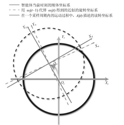
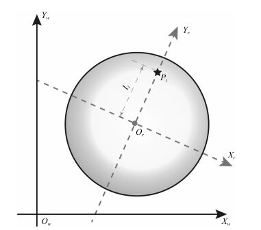
    图  2  $λ_i(t)$ 与 $\widetilde{λ}_i(t)$ 近似关系示意图

    Fig.  2  Diagram of approximate relationship between $λ_i(t)$ and $\widetilde{λ}_i(t)$
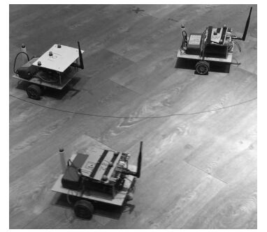
    图  3  实验用差分驱动轮式机器人照片

    Fig.  3  A photo of experimental differentially driven wheeled mobile robots

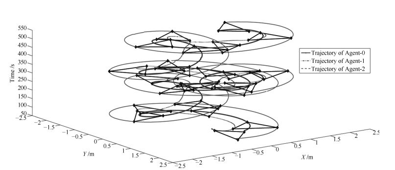
    图  4  三角形编队实验中各智能体的运动轨迹

    Fig.  4  Trajectories of agents in experiments presented in triangle formation

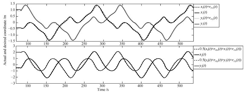
    图  5  三角形编队实验中智能体 $1$ 和智能体 $2$ 对期望队形的跟踪效果

    Fig.  5  Tracking performance of Agent $1$ and Agent $2$ in triangle formation experiment
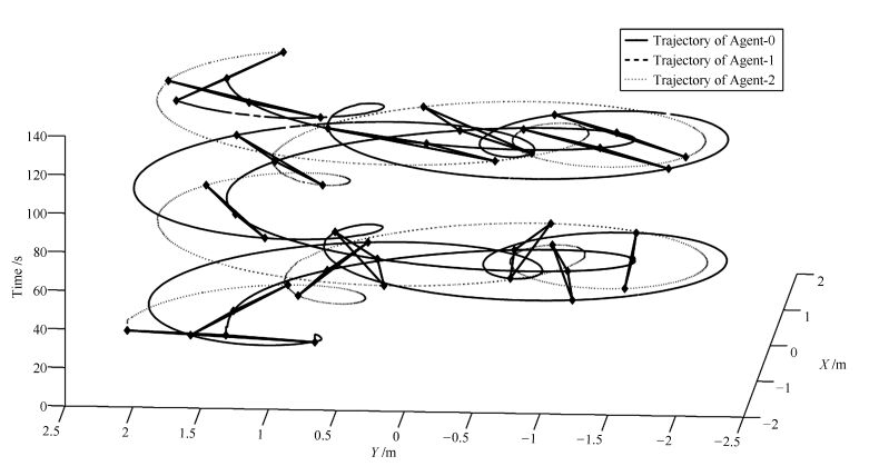
    图  6  环绕编队中各智能体的轨迹

    Fig.  6  Trajectories of agents in the surrounding formation experiment

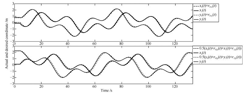
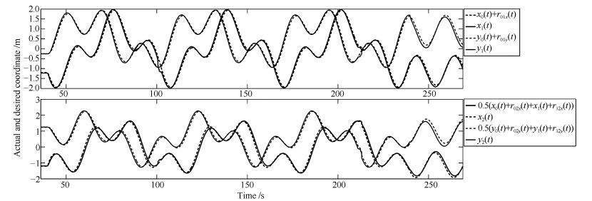
    图  7  环绕编队中各智能体对期望的队形的跟踪性能

    Fig.  7  Tracking performance of agents on desired formation in the surrounding formation experiment

    图  8  经过偏移后的环绕编队中各智能体的跟踪性能

    Fig.  8  Tracking performance of agents on desired formation in the transferred surrounding formation experiment

  • [1] 张晓平, 阮晓钢, 肖尧, 朱晓庆.两轮机器人具有内发动机机制的感知运动系统的建立.自动化学报, 2016, 42(8):1175-1184 http://www.aas.net.cn/CN/abstract/abstract18907.shtml

    Zhang Xiao-Ping, Ruan Xiao-Gang, Xiao Yao, Zhu Xiao-Qing. Establishment of a two-wheeled robot's sensorimotor system with mechanism of intrinsic motivation. Acta Automatica Sinica, 2016, 42(8):1175-1184 http://www.aas.net.cn/CN/abstract/abstract18907.shtml
    [2] 董文杰, 霍伟.受非完整约束移动机器人的跟踪控制.自动化学报, 2000, 26(1):1-6 http://www.aas.net.cn/CN/abstract/abstract16055.shtml

    Dong Wen-Jie, Huo Wei. Tracking control of mobile robots with nonholonomic constraint. Acta Automatica Sinica, 2000, 26(1):1-6 http://www.aas.net.cn/CN/abstract/abstract16055.shtml
    [3] 闵海波, 刘源, 王仕成, 孙富春.多个体协调控制问题综述.自动化学报, 2012, 38(10):1557-1570 http://www.aas.net.cn/CN/abstract/abstract17765.shtml

    Min Hai-Bo, Liu Yuan, Wang Shi-Cheng, Sun Fu-Chun. An overview on coordination control problem of multi-agent system. Acta Automatica Sinica, 2012, 38(10):1557-1570 http://www.aas.net.cn/CN/abstract/abstract17765.shtml
    [4] Velasco-Villa M, Castro-Linares R, Rosales-Hernández F, del Muro-Cuéllar B, Hernández-Pérez M A. Discrete-time synchronization strategy for input time-delay mobile robots. Journal of the Franklin Institute, 2013, 350(10):2911-2935 doi: 10.1016/j.jfranklin.2013.05.029
    [5] Rosales-Hernández F, Velasco-Villa M, Castro-Linares R, del Muro-Cuéllar B, Hernández-Pérez M Á. Synchronization strategy for differentially driven mobile robots:discrete-time approach. International Journal of Robotics and Automation, 2015, 30(1):50-59 https://www.researchgate.net/profile/Rafael_Castro-Linares/publication/277941042_Synchronization_strategy_for_differentially_driven_mobile_robots_Discrete-time_approach/links/5604293608aea25fce30b9f2.pdf?origin=publication_list
    [6] Dong W J, Djapic V. Leader-following control of multiple nonholonomic systems over directed communication graphs. International Journal of Systems Science, 2016, 47(8):1877-1890 doi: 10.1080/00207721.2014.955553
    [7] Peng Z X, Yang S C, Wen G G, Rahmani A, Yu Y G. Adaptive distributed formation control for multiple nonholonomic wheeled mobile robots. Neurocomputing, 2016, 173(P3):1485-1494 https://www.researchgate.net/publication/282409600_Adaptive_Distributed_Formation_Control_for_Multiple_Nonholonomic_Wheeled_Mobile_Robots
    [8] Cepeda-Gomez R, Perico L F. Formation control of nonholonomic vehicles under time delayed communications. IEEE Transactions on Automation Science and Engineering, 2015, 12(3):819-826 doi: 10.1109/TASE.2015.2424252
    [9] Dong X W, Zhou Y, Ren Z, Zhong Y S. Time-varying formation control for unmanned aerial vehicles with switching interaction topologies. Control Engineering Practice, 2016, 46:26-36 doi: 10.1016/j.conengprac.2015.10.001
    [10] Wang R, Dong X W, Li Q D, Ren Z. Distributed adaptive time-varying formation for multi-agent systems with general high-order linear time-invariant dynamics. Journal of the Franklin Institute, 2016, 353(10):2290-2304 doi: 10.1016/j.jfranklin.2016.03.016
    [11] Bai J, Wen G G, Rahmani A, Chu X, Yu Y G. Consensus with a reference state for fractional-order multi-agent systems. International Journal of Systems Science, 2016, 47(1):222-234 doi: 10.1080/00207721.2015.1056273
    [12] Wang C, Sun D. A synchronous controller for multiple mobile robots in time-varied formations. In:Proceedings of the 2008 IEEE/RSJ International Conference on Intelligent Robots and Systems. Nice, France:IEEE, 2008. 2765-2770
    [13] Brinon-Arranz L, Seuret A, Canudas-de-Wit C. Cooperative control design for time-varying formations of multi-agent systems. IEEE Transactions on Automatic Control, 2014, 59(8):2283-2288 doi: 10.1109/TAC.2014.2303213
    [14] Ferrers N M. Extension of Lagrange's equations. Journal of Pure and Applied Mathematics, 1872, 12(45):1-5 http://www.ams.org/bull/1932-38-02/S0002-9904-1932-05342-3/S0002-9904-1932-05342-3.pdf
    [15] Khooban M H. Design an intelligent proportional-derivative (PD) feedback linearization control for nonholonomic-wheeled mobile robot. Journal of Intelligent & Fuzzy Systems, 2014, 26(4):1833-1843 https://www.deepdyve.com/lp/ios-press/design-an-intelligent-proportional-derivative-pd-feedback-xTHDTVhiJw
    [16] Oriolo G, De Luca A, Vendittelli M. WMR control via dynamic feedback linearization:design, implementation, and experimental validation. IEEE Transactions on Control Systems Technology, 2002, 10(6):835-852 doi: 10.1109/TCST.2002.804116
    [17] Rudra S, Barai R K, Maitra M. Design and implementation of a block-backstepping based tracking control for nonholonomic wheeled mobile robot. International Journal of Robust and Nonlinear Control, 2016, 26(14):3018-3035 doi: 10.1002/rnc.3485
    [18] Velazquez M, Cruz D, Garcia S, Bandala M. Velocity and motion control of a self-balancing vehicle based on a cascade control strategy. International Journal of Advanced Robotic Systems, 2016, 13(3):Article No.1061 http://www.intechopen.com/journals/statistics/international_journal_of_advanced_robotic_systems/velocity-and-motion-control-of-a-self-balancing-vehicle-based-on-a-cascade-control-strategy
    [19] Wikipedia. Breadth-first/search[Online], available:https://en.wikipedia.org/wiki/Breadth-first_search, November 10, 2016.
    [20] Zhao J, Liu G P. Model-based remote control of nonholonomic wheeled robot with time delay and packet loss in forward channel. In:Proceedings of the 2015 Chinese Automation Congress. Wuhan, China:IEEE, 2015. 1669-1704
  • 期刊类型引用(5)

    1. 闫辉,贾彦茹,董建军. 一种两轮自平衡机器人比例-积分-微分控制方法. 自动化技术与应用. 2021(03): 6-10 . 百度学术
    2. 孙玉娇,杨洪勇,于美妍. 基于领航者的多机器人系统编队控制研究. 鲁东大学学报(自然科学版). 2020(01): 35-39+97 . 百度学术
    3. 王雅. 多智能体系统的包含控制研究. 电子技术与软件工程. 2020(11): 30-33 . 百度学术
    4. 杨彬,周琪,曹亮,鲁仁全. 具有指定性能和全状态约束的多智能体系统事件触发控制. 自动化学报. 2019(08): 1527-1535 . 本站查看
    5. 张文,马忠军,王毅. 带未知耦合权重的领导—跟随多智能体系统的实用一致性. 自动化学报. 2018(12): 2300-2304 . 本站查看

    其他类型引用(10)

  • 加载中
  • 图(8)
    计量
    • 文章访问数:  2889
    • HTML全文浏览量:  344
    • PDF下载量:  850
    • 被引次数: 15
    出版历程
    • 收稿日期:  2016-08-25
    • 录用日期:  2016-11-23
    • 刊出日期:  2017-07-20

    目录

    /

    返回文章
    返回