

-
摘要: 为满足新颖成像模式对卫星姿态快速机动或对规划姿态的高精度跟踪控制需求,本文针对金字塔构型控制力矩陀螺(Control moment gyroscopes,CMG)群与反作用飞轮为联合执行机构的挠性敏捷卫星,提出一种融合以Legendre伪谱法实现卫星姿态及CMG群框架角速度最优规划的前馈控制、以非线性模型预测控制(Nonlinear model predictive control,NMPC)实现最优轨迹反馈跟踪的复合控制方法.在前馈控制律设计中,充分考虑了CMG群的力矩输出能力、奇异性及振动抑制性能等约束,规划获得了最优的CMG群框架角速度、卫星的姿态角及角速度.在反馈控制律设计中,以飞轮输出力矩能力、姿态机动快速性及能量为约束,设计了具有滚动优化思想的跟踪算法,补偿由于初始状态及转动惯量偏差等带来的控制误差.研究结果表明,在转动惯量存在偏差情况下,本文的控制方法仍是有效的,且表现出较强的鲁棒性.Abstract: To satisfy the needs of novel imaging modes for attitude rapid maneuver and high precision tracking control, a control strategy combining feedforward and feedback control is proposed for flexible satellite with hybrid actuator (pyramid configuration control moment gyroscopes (CMG) and reaction flywheel). In the design of feedforward control, to fully consider the constraints, such as torque output capacity of CMG group, singularity and vibration suppression performance, a Legendre pseudospectral method which could plan the optimal satellite attitude and frame angle rate of CMG group is presented. In the design of feedback control, with the torque capacity of flywheel, attitude rapid maneuver and energy constraints being the cost function, a tracking control algorithm based on nonlinear model predictive control (NMPC) is given to compensate the error of initial state and rotational inertia. The results show that, in the case of inertia error, the proposed control method is effective and shows a strong robustness.
-
Key words:
- Agile satellite /
- rapid maneuver /
- hybrid actuator /
- trajectory optimization /
- moving horizon tracking
-
1. Introduction
Since recent few decades, some researchers focus their energy on the robust stability and controller design problems about the networked-control systems (NCSs) with some uncertain parameters because some networked-control systems have been succeeded in applications in modern complicated industry processes, e.g., aircraft and space shuttle, nuclear power stations, high-performance automobiles, etc. The fuzzy-logic control based on the Takagi-Sugeno (T-S) is widely used to dealing with complex nonlinear systems because it has simple dynamic structure and highly accurate approximation to any smooth nonlinear function in any compact set. One can consult [1]$-$[8] and the other cited literature therein [9]$-$[31]. Data-packet dropout is an important issue to be addressed in the networked-control systems [6], [32]. Zhang [33] solves the problem of $H_\infty$ estimation for a class of Markov jump linear systems but he neglect possible dropout in practice. Reference [34] reports the problem of $H_\infty$ stability of discrete-time switched linear system with average dwell time and with no dropout. In [6], piecewise Lyapunov function is proposed to analyze robust of the nonlinear NCSs without time-delay issue. Random data-packet dropout and time delay are well considered but the controlled NCSs are linear systems in [32]. Reference [8] discusses the problem of robust $H_\infty$ output feedback control for a class of continuous-time Takagi-Sugeno (T-S) fuzzy affine dynamic systems with parametric uncertainties and input constraints on ignoring some nonlinearities induced by system with data-packet dropout and random time delay. Reference [5] investigates the robust $H_\infty$ stability of a class of half nonlinear NCSs with multiple probabilistic delays and multiple missing measurements regardless of the dropout in the forward path. According to above consideration, we investigate a class of new nonlinear NCSs, in which not only sensors communicate with controllers by network but also controllers do with actuator in the same manner.
The highlights of this paper, which lie primarily on the new research problems and new system models, are summarized as follows:
1) A new model is established, in which the controllers communicate with the actuator by a wireless network and the random missing control from the controller to the actuator occurs and the sensors do with the controllers in the same manner.
2) The investigation on the T-S fuzzy model is used for a class of complex systems that describe the modeling errors, disturbance rejection attenuation, probabilistic delay, missing measurements and missing control within the same framework.
The rest of this paper is organized as follows. The problem under consideration is formulated in Section 2. Development of robust $H_{\infty}$ fuzzy control performance on the exponentially stability the closed-loop fuzzy system are placed in Section 3. Section 4 gives design of robust $H_\infty$ fuzzy controller. An illustrative example is given in Section 5, and we conclude the paper in Section 6.
Notation 1: The notation used in the paper is fairly standard. %The superscript "T" stands for matrix transpose; $\mathbb{R}^n$ denotes the $n$-dimensional real vectors; $\mathbb{R}^{m\times n}$ denotes the $n$-dimensional matrix; and $I$ and 0 represent the identity matrix and zero matrix, respectively. The notation $P>0$ ($P\geq 0$) means that $P$ is real symmetric and positive definite (semi-definite), ${\rm tr}(M)$ refers to the trace of the matrix $M$, and $ \|\cdot\|_2 $ stands for the usual $l_2$ norm. In symmetric block matrices or complex matrix expressions, we use an "$\star$" to represent a term that is induced by symmetry, and ${\rm diag}\{\cdots\}$ stands for a block-diagonal matrix. In addition, ${E}\{x\}$ and ${E}\{x|y\}$ will, respectively, mean expectation of $x$ and expectation of $x $ conditional on $y$.
2. Problem Formulation
In this note, the output feedback control problem for discrete-time fuzzy systems in NCSs is taken in our consideration, where the frame-work is depicted in Fig. 1.
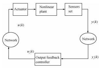 图 1 Framework of output feedback control systems over network environment.Fig. 1 Framework of output feedback control systems over network environment.
The sensors are connected to a network, which are shared by other NCSs and susceptible to communication delays and missing measurements or pack dropouts). As Fig. 1 depicts, pack dropouts from the controller to actuator can take place stochastically. The fuzzy systems with multiple stochastic communication delays and uncertain parameters can be read as follows:
Plant Rule $i$: If $\theta_{1}(k) $ is $ M_{i1}$, and $\theta_{2}(k)$ is $M_{i2}$, and, $\ldots$, and $\theta_{p}(k)$ is $M_{ip}$, then
$ \begin{align} x(k+1)=&\ A_i(k)x(k)+A_{di}\sum\limits_{m=1}^{h}\alpha_m(k)x(k-\tau_m(k))\notag\\ & +B_{1i}u(k)+D_{1i}v(k)\notag\\ \tilde{y}(k)=&\ C_ix(k)+D_{1i}v(k)\notag\\ z(k)=&\ C_{zi}(k)+B_{2i}u(k)+D_{3i}v(k)\notag\\ x(k)=&\ \phi(k)\quad\forall\, {k}\in \mathbb{Z}^{-}, ~\, i=1, \ldots, r \end{align} $
(1) where $M_{ij}$ is the fuzzy set, $r$ stands for the number of If-then rules, and $\theta(k)=[\theta_1(k), \theta_2(k), \ldots, \theta_{p}(k)]$ is the premise variable vector, which is independent of the input variable $u(k)$. $x(k)\in \mathbb{R}^n$ is the state vector, $u(k)\in \mathbb{R}^m$, $\tilde{y}$ $\in$ $\mathbb{R}^s$ is the process output, $z(k)\in \mathbb{R}^q$ is the controlled output, $v(k)\in \mathbb{R}^p$ presents a vector of exogenous inputs, which belongs to $l_2[0, \infty)$, $\tau_m(k)$ $(m=1, 2, \ldots, h)$ are the communication delays that vary with the stochastic variables $\alpha_m(k)$, and $\phi(k)$ $(\forall\, {k}\in \mathbb{Z}^{-})$ is the initial state.
The stochastic variables $\alpha_m(k)\in \mathbb{R}$ $(m=1, 2, \ldots, h)$ in (1) are assumed to satisfy mutually uncorrelated Bernoulli-distributed-white sequences described as follows:
$ \begin{align} & {\rm Prob}\{\alpha_m(k)=1\}={E}\{\alpha_m(k)\}=\bar{\alpha}_m\notag\\ & {\rm Prob}\{\alpha_m(k)=0\}=1-\bar{\alpha}_m.\notag \end{align} $
In this note, one can make the random communication-time delays satisfy the following assumption that the time-varying $\tau_m(k)$ $ (m=1, 2, \ldots, h)$ are subject to $ d_t\leq \tau_m(k)$ $\leq$ $d_T$. The matrices $A_i(k)=A_i+\Delta{A_i(k)}$, $C_{zi}(k)= C_{zi}$ $+$ $\Delta{C_{zi}}(k)$, where $ A_i, A_{di}, B_{1i}, B_{2i}, C_i, C_{zi}, D_{1i}, D_{2i}$, and $D_{3i}$ are known constant matrices with compatible dimensions. $\Delta{A_i(k)} $ and $\Delta C_{zi}(k)$ with the time-varying norm-bounded uncertainties satisfy
$ \begin{align} \left[ \begin{array}{c} \Delta A_i(k)\\ \Delta C_{zi}(k)\\ \end{array} \right]=\left[ \begin{array}{c} H_{ai}\\ H_{ci}\\ \end{array} \right]F(k)E \end{align} $
(2) with $H_{ai}$, $H_{ci}$ being constant matrices and $F^T(k)F(k)\leq I$, $\forall\, {k}$.
In this note, the packet dropout (the miss-measurement) read as
$ \begin{align} y_c(k)&= \Xi{C_i}x(k)+D_{2i}(k)\notag\\ &=\sum\limits_{l=1}^{s}\beta_lC_{il}x(k)+D_{2i}v(k)\notag\\ u(k)&=W(k)u_c(k)=W(k)C_{ki}x_c(k) \end{align} $
(3) where $\Xi=\hbox{diag}\{\beta_1, \ldots, \beta_s\}$ with $\beta_l$ $(l=1, 2, \ldots, s)$ being $s$ unrelated random variables, which are also unrelated with $\alpha_m(k)$ and $W(k)$ denoting the random packet missing from the controllers to the actuator. One can assume that $\beta_l $ has the probabilistic-density function $q_l(s)$ $(l=1, 2, \ldots, s)$ on the interval $[0, 1]$ with mathematical expectation $\mu_l$ and variance $\sigma_l^2$. $C_{il}={\rm diag}\{\underbrace{0, \ldots, 0}\limits_{l-1}, 1, \underbrace{0, \ldots, 0}\limits_{s-l}\}C_i$. We denote the stochastic pack dropouts from the controller to the actuator by $W(k)= {\rm diag}\{\omega_1(k), \ldots, \omega_m(k)\}$, where $\omega_l$ $(l=$ $1, 2, \ldots, m)$ are mutually unrelated random variables and obey Bernoulli distribution with mathematical expectation $\bar{\omega}_l$ and variance$\rho_l $and assumed to be unrelated with $\alpha_m(k)$. For a given pair of $(x(k), u(k))$, the final output of the fuzzy system is read as
$ \begin{align} x(k+1)=&\, \sum\limits_{i=1}^{r}h_i(\theta(k))[A_i(k)x(k)+B_{1, i}u(k)\notag\\ &\, +A_{di}\sum\limits_{m=1}^{h}x(k-\tau_m(k))+D_{1i}v(k)]\notag\\ y_c(k)=&\, \sum\limits_{i=1}^{r}h_i(\theta(k))[\Xi{C_i}x(k)+D_{2i}v(k)]\notag\\ z(k)=&\, \sum\limits_{i=1}^{r}h_i(\theta(k))[C_{zi}(k)x(k)+B_{2i}u(k)+D_{3i}v(k)] \end{align} $
(4) where the fuzzy-basis functions are described as
$ \begin{align} &{h_i(\theta(k))}=\frac {\vartheta_i(\theta(k))} {\sum\limits_{i=1}^{r}\vartheta_i(\theta(k))}\notag\\ &\vartheta_i(\theta(k))=\prod\limits_{j=1}^{p}M_{ij}(\theta_j(k))\notag \end{align} $
with $M_{ij}(\theta_j(k))$ being the grade of membership of $\theta_j(k)$ in $M_{ij}$. It is clear that $\vartheta_i(\theta(k))\geq 0$, $i=1, 2, \ldots, r$, $\sum_{i=1}^{r}\vartheta_i(\theta(k))>0$, $\forall\, {k}$, and $h_i(\theta(k))\geq 0$, $i=1, 2, \ldots, r$, $\sum_{i=1}^{r}h_i(\theta(k))=1$, $\forall\, {k}$. In the sequel, we denote $h_i=h_i(\theta(k))$ for brevity.
In the note, the fuzzy dynamic output-feedback controller for the fuzzy system (4) is given as
Controller Rule $i$: If $\theta_1(k)$ is $M_{il}$ and $\theta_2(k)$ is $M_{i2}$ and, $\ldots$, and $\theta_p(k)$ is $M_{ip}$ then
$ \begin{align} \begin{cases} x_c(k+1)=A_{ki}x_c(k)+B_{ki}y_c(k)\\ u(k)= W(k)C_{ki}x_c(k) \end{cases} \end{align} $
(5) with $x_c(k)\in \mathbb{R}^n$ being the controller state along with the controller parameters $A_{ki}$, $B_{ki}$ and $C_{ki}$ to be determined. Naturally, the overall fuzzy output-feedback controller is read as
$ \begin{align} \begin{cases} x_c(k+1)=\sum\limits_{i=1}^{r}h_i[A_{ki}x_c(k)+B_{ki}y(k)]\\ u(k)=\sum\limits_{i=1}^{r}h_iW(k)C_{ki}x_c(k), \ \ i=1, 2, \ldots, r. \end{cases} \end{align} $
(6) Combining (6) with (4), we can obtain the closed-loop system described as
$ \begin{align} \begin{cases} \bar{x}(k+1)=\sum\limits_{i-1}^{r}\sum\limits_{j=1}^{r}h_ih_j[(A_{ij}+B_{ij})\bar{x}(k)+D_{ij}v(k) \\ \qquad \qquad \quad\, +\sum\limits_{m=1}^{h}(\bar{A}_{dmi}+\tilde{A}_{dmi})\bar{x}(k-\tau_m(k)]\\ z(k)=\sum\limits_{i=1}^{r}\sum\limits_{j=1}^{r}h_ih_j[\bar{C}_{ij}(k)+\bar{\bar{C}}_{ij}]\bar{x}(k) +D_{3i}v(k) \end{cases} \end{align} $
(7) where
$ \begin{align*} &\bar{x}(k)=\left[ \begin{array}{c} x(k) \\ x_c(k) \\ \end{array} \right], \quad A_{ij}=\left[ \begin{array}{cc} A_i(k)&B_{1i}\bar{W}C_{kj} \\ B_{ki}\bar{\Xi}C_j&A_{ki} \\ \end{array} \right]\\[1mm] &B_{ij}=\left[ \begin{array}{cc} 0& B_{1i}\tilde{W}(k)C_{kj}\\ B_{ki}\tilde{\Xi}C_j& 0\\ \end{array} \right]\\[1mm] &\bar{A}_{dmi}=\left[ \begin{array}{cc} \bar{\alpha}_mA_{di}&0 \\ 0&0 \\ \end{array} \right], \quad \tilde{A}_{dmi}=\left[ \begin{array}{cc} \tilde{\alpha}_mA_{di}&0 \\ 0&0 \\ \end{array} \right]\\[1mm] &D_{ij}=\left[ \begin{array}{c} D_{1i} \\ B_{ki}D_{2j} \\ \end{array} \right], \quad \bar{C}_{ij}(k)=\bigg[ \begin{array}{cc} C_{zi}(k)&B_{2i}\bar{W}C_{kj} \\ \end{array} \bigg]\\[1mm] &\bar{\bar{C}}_{ij}(k)=\bigg[ \begin{array}{cc} 0&B_{2i}\tilde{W}(k)C_{kj} \\ \end{array} \bigg] \end{align*} $
with $\tilde{\alpha}_m(k)=\alpha_m(k)-\bar{\alpha}_m(k)$ and $\tilde{\omega}_j(k)={\omega}_j(k)-\bar{\omega}_j(k)$. It is evident that $E\{\tilde{\alpha}_m(k)\}=0$ and that $E\{\tilde{\omega}_j(k)\}=0$ and that $E\{\tilde{\alpha}_m^2(k)\}=\bar{\alpha}_m(1-\bar{\alpha}_m)=\sigma_m^2$ and that $E\{\tilde{\omega}_j^2(k)\}$ $=$ $\bar{\omega}_j(1-\bar{\omega}_j)=\rho_j^2$.
Denote
$ \begin{align*} &\bar{x}(k-\tau)\\ &=\left[ \!\!\begin{array}{cccc} \ \ \bar{x}^T(k-\tau_1(k)) &\!\bar{x}^T(k-\tau_2(k))&\! \cdots &\!\bar{x}^T(k-\tau_h(k))\ \ \\ \end{array} \!\!\right]^T\\ &\xi(k)=\left[ \begin{array}{ccc} \bar{x}^T(k)&\bar{x}^T(k-\tau) &v^T(k) \\ \end{array} \right]^T\end{align*} $
then (7) can also be rewritten as
$ \begin{align} \begin{cases} \bar{x}(k+1) =\sum\limits_{i=1}^{r}\sum\limits_{j=1}^{r}h_ih_j\left[A_{ij}\!+B_{ij}, \hat{Z}_{mi}\!+\Delta\hat{Z}_{mi}, D_{ij}\right]\xi(k) \\ z(k)=\sum\limits_{i=1}^{r}\sum\limits_{j=1}^{r}h_ih_j\left[\bar{C}_{ij}+ \bar{\bar{C}}_{ij}, 0, D_{3i}\right]\xi(k) \end{cases} \end{align} $
(8) where $\hat{Z}_{mi}=[\bar{A}_{d1i}, \ldots, \bar{A}_{dhi}]$ and $\Delta\hat{Z}_{mi}=[\tilde{A}_{d1i}, \ldots, \tilde{A}_{dhi}]$. In order to smoothly formulate the problem in the note, we introduce the following definition.
Definition 1: For the system (7) and every initial conditions $\phi$, the trivial solution is said to be exponentially mean square stable if, in the case of $v(k)=0$, there exist constants $\delta>0$ and $0<\kappa<1$ such that $E\{\|\bar{x}(k)\|^2\}$ $\leq$ $\delta\kappa^k \sup_{-d_M\leq i\leq 0}E\{\|{\phi(i)}\|^2\}$, $\forall\, {k}\geq 0$.
We will develop techniques to settle the robust $H_{\infty}$ dynamic output feedback problem for the discrete-time fuzzy system (7) subject to the following conditions:
1) The fuzzy system (7) is exponentially stable in the mean square.
2) Under zero-initial condition, the controlled output $z(k)$ satisfies
$ \begin{align} \sum\limits_{k=0}^{\infty}E\left\{\|{z(k)}\|^2\right\}\leq \gamma^2\sum\limits_{k=0}^{\infty}E\left\{\|{v(k)}\|^2\right\} \end{align} $
(9) for all nonzero $v(k)$, where $\gamma>0$ is a prescribed scalar.
Remark 1: The proposed new model has the function that not only the controllers communicate with the actuator by wireless but also the sensors do with the controllers by the same manner.
3. Development of Robust ${\pmb H}_{\pmb \infty}$ Fuzzy Control Performance
At first, we give the following lemma, which will be adopted in obtaining our main results.
Lemma 1 (Schur complement): Given constant matrices $S_1$, $S_2$, $S_3$, where $S_1=S_1^T$ and $0<S_2=S_2^T$, then $ S_1$ $+$ $S_3^TS_2^{-1}S_3$ $<$ $0$ if and only if
$ \begin{align*} \left[ \begin{array}{cc} S_1&S_3^T \\ S_3 &-S_2 \\ \end{array} \right]<0~~ \hbox{or}~~ \left[ \begin{array}{cc} -S_2&S_3 \\ S_3^T&S_1 \\ \end{array} \right]<0. \end{align*} $
Lemma 2 (S-procedure) [5]: Letting $L=L^T$ and $H$ and $E$ be real matrices of appropriate dimensions with $F$ satisfying $FF^T\leq I$, then $ L+HFE+E^TF^TH^T<0$ if and only if there exists a positive scalar $\varepsilon>0$ such that $L$ $+$ $\varepsilon^{-1}HH^T+\varepsilon E^TE<0$, or equivalently
$ \begin{align*} \left[ \begin{array}{ccc} L&H&\varepsilon{E^T} \\ H^T &-\varepsilon{I}&0 \\ \varepsilon{E}&0 &-\varepsilon{I} \\ \end{array} \right]<0. \end{align*} $
Lemma 3: For any real matrices $X_{ij}$ for $i$, $j=1, 2, \ldots, $ $r$ and $n>0$ with appropriate dimensions, we have [35]
$ \sum\limits_{i=1}^r\sum\limits_{j=1}^r\sum\limits_{l=1}^r\sum\limits_{l=1}^rh_ih_jh_kh_lX_{ij}^T\Lambda{X_{kl}}\leq\sum\limits_{i=1}^r\sum\limits_{j=1}^rh_ih_jX_{ij}^T\Lambda X_{ij}. $
Theorem 1: For given controller parameters and a prescribed $H_{\infty}$ performance $\gamma>0$, the nominal fuzzy system (7) is exponentially stable if there exist matrices $P>0$ and $Q_k$ $>$ $0$, $k=1, 2, \ldots, h$, satisfying
$ \left[ \begin{array}{cc} \Pi_i&\star \\ 0.5\Sigma_{ii}&\bigwedge \\ \end{array} \right]<0 $
(10) $ \left[ \begin{array}{cc} 4\Pi_i&\star \\ \Sigma_{ij}&\bigwedge \\ \end{array} \right]<0, \quad 1\leq i<j\leq r $
(11) where
$ \Pi_i =\ {\rm diag}\bigg\{-P+\sum\limits_{k=1}^h(d_T-d_t+1)Q_k, \hat{\alpha}\breve{A}_{di}^T\breve{P} \breve{A}_{di}\notag\\ \ \ \ \ \ \ -{\rm diag}\{Q_1, Q_2, \ldots, Q_h\}, -\gamma^2I\bigg\} $
(12) $\begin{align*} \hat{\alpha}=&\ {\rm diag}\left\{\bar{\alpha}_1(1-\bar{\alpha}_1), \ldots, \bar{\alpha}_h(1-\bar{\alpha}_h)\right\}\notag\\ \breve{A}_{di}=&\ {\rm diag}\{\underbrace{\hat{A}_{di}, \ldots, \hat{A}_{di}}\limits_h\}\notag\\ \check{C}_{ij}=&\ \left[\sigma_1\hat{C}_{11ij}^TP, \ldots\!, \sigma_s\hat{C}_{1sij}^TP, \rho_1\hat{C}_{k1ij}^TP, \ldots\!, \rho_m\hat{C}_{kmij}^TP\right]^T\notag\\ &\check{P}=\hbox{diag}\{\underbrace{P, \ldots, P}\limits_{s+m}\}\\ &{\small\bigwedge}=\hbox{diag}\{-\check{P}, -P, -I, \hbox{diag}\{\underbrace{-I, \ldots, -I}\limits_m\}\}\\ &\breve{P}=\hbox{diag}\{\underbrace{P, \ldots, P}\limits_h\}\\ &\hat{A}_{di}=\left[ \begin{array}{cc} A_{di}&0\\ 0&0\\ \end{array} \right] \\ &\Sigma_{ij}=\\ &\!\!\!\left[\!\!{\small \begin{array}{ccccc} \check{C}_{ij}\!+\!\check{C}_{ji}\! &\! 0\!&\!0 \\[2mm] PA_{ij}\!+\!PA_{ji} \! &\! P\hat{Z}_{mi}\!+\!P\hat{Z}_{mj} \! &\!PD_{ij}\!+\!PD_{ji}\\[2mm] \bar{C}_{ij}\!+\!\bar{C}_{ji}\! &\!0\! &\!D_{3i}\!+\!D_{3j}\\[2mm] \, [0 ~~ \rho_1B_{2i}C_{kj1}\!+\!\rho_1B_{2j}C_{ki1}] \! &\!0\! &\!0\\[2mm] \vdots\! &\!\vdots\! &\!\vdots\\[2mm] \, [0 ~~ \rho_mB_{2i}C_{kjm}\!+\!\rho_mB_{2j}C_{kim}]\! &\!0\! &\!0\\ \end{array}}\!\!\!\! \right]. \end{align*} $
Proof:
Let
$ \begin{align*} &\Theta_j(k)=\{x(k-\tau_j(k), x(k-\tau_j(k)+1, \ldots, x(k)\}\\ &\chi(k)=\{\Theta_1(k)\bigcup\Theta_2(k)\bigcup\ldots\bigcup\Theta_h(k)\}=\bigcup\limits_{j=1}^{h}\Theta_j(k) \end{align*} $
where $j=1, 2, \ldots, h$. We consider the following Lyapunov functional for the system of (7): $V(\chi(k))=\sum_{i=1}^3V_i(k)$, where
$ \begin{align*} &V_1(k)=\bar{x}^T(k)P\bar{x}\\ &V_2(k)=\sum\limits_{j=1}^{h}\sum\limits_{i=k-\tau_j(k)}^{k-1}\bar{x}^T(i)Q_j\bar{x}(i)\\ &V_3(k)=\sum\limits_{j=1}^h\sum\limits_{m=-d_M+1}^{-d_m}\sum\limits_{i=k+m}^{k-1}\bar{x}^T(i)Q_j\bar{x}(i) \end{align*} $
with $P>0$, $Q_j>0$ $(j=1, 2, \ldots, h)$ being matrices to be determined.
$ \begin{align} {E}[\Delta{V}|x(k)]&={E}[V(\chi(k+1))|\chi(k)]-V(\chi(k))\notag\\ & ={E}[(V(\chi(k+1))-V(\chi(k)))|\chi(k)]\notag\\ & =\sum\limits_{i=1}^{3}{E}[\Delta{V_i}|\chi(k)]. \end{align} $
(13) According to (7), we have
$ \begin{align*} &{E}\{\Delta{V_1}|\chi(k)\}\\ &\qquad={E} \left[(\bar{x}^T(k+1)P\bar{x}(k+1)-\bar{x}^T(k)P\bar{x}(k))|\chi(k)\right]\\ &\qquad\leq\xi^T(k)\sum\limits_{i=1}^{r}\sum\limits_{j=1}^{r}\Omega_{ij}\xi(k) \end{align*} $
where
$ \begin{align} & {{\Omega }_{ij}}=E\left\{ \left[\begin{matrix} A_{ij}^{T}P{{A}_{ij}}+B_{ij}^{T}P{{B}_{ij}}-P & {} \\ \star & {} \\ \star & {} \\ \end{matrix} \right. \right. \\ & \left. \left. \begin{matrix} {} & A_{ij}^{T}P{{{\hat{Z}}}_{mi}} & A_{ij}^{T}P{{D}_{ij}} \\ {} & \hat{Z}_{mi}^{T}P{{{\hat{Z}}}_{mi}}+\Delta \hat{Z}_{mi}^{T}P\Delta {{{\hat{Z}}}_{mi}} & \hat{Z}_{mi}^{T}P{{D}_{ij}} \\ {} & \star & D_{ij}^{T}P{{D}_{ij}} \\ \end{matrix} \right] \right\} \\ \end{align} $
$ {{B}_{ij}}=\left[\begin{matrix} 0 & 0 \\ {{B}_{ki}}\tilde{\Xi }{{C}_{j}} & 0 \\ \end{matrix} \right]+\left[\begin{matrix} 0 & {{B}_{1i}}\tilde{\omega }(k){{C}_{kj}} \\ 0 & 0 \\ \end{matrix} \right] $
$ \begin{align} & E\{B_{ij}^{T}P{{B}_{ij}}\} \\ & \ \ \ \ \ =\sum\limits_{l=1}^{s}{\sigma _{l}^{2}}{{\left[\begin{matrix} 0 & 0 \\ {{B}_{ki}}{{C}_{jl}} & 0 \\ \end{matrix} \right]}^{T}}P\left[\begin{matrix} 0 & 0 \\ {{B}_{ki}}{{C}_{jl}} & 0 \\ \end{matrix} \right] \\ & \ \ \ \ \ +\sum\limits_{l=1}^{m}{\rho _{l}^{2}}{{\left[\begin{matrix} 0 & {{B}_{1i}}{{C}_{kjl}} \\ 0 & 0 \\ \end{matrix} \right]}^{T}}P\left[\begin{matrix} 0 & {{B}_{1i}}{{C}_{kjl}} \\ 0 & 0 \\ \end{matrix} \right] \\ & \ \ \ ={{({{{\overset{\lower0.5em\hbox{$\smash{\scriptscriptstyle\smile}$}}{P}}}^{-1}}{{{\overset{\lower0.5em\hbox{$\smash{\scriptscriptstyle\smile}$}}{C}}}_{lij}})}^{T}}\overset{\lower0.5em\hbox{$\smash{\scriptscriptstyle\smile}$}}{P}({{{\overset{\lower0.5em\hbox{$\smash{\scriptscriptstyle\smile}$}}{P}}}^{-1}}{{{\overset{\lower0.5em\hbox{$\smash{\scriptscriptstyle\smile}$}}{C}}}_{lij}}) \\ \end{align} $
$ \begin{align} & \overset{\lower0.5em\hbox{$\smash{\scriptscriptstyle\smile}$}}{P}=\rm{diag}\{\underbrace{\mathit{P}, \ldots, \mathit{P}}_{\mathit{s}+\mathit{m}}\} \\ & {{{\hat{C}}}_{1lij}}=\left[\begin{matrix} 0 & 0 \\ {{B}_{ki}}{{C}_{jl}} & 0 \\ \end{matrix} \right] \\ & {{{\hat{C}}}_{klij}}=\left[\begin{matrix} 0 & {{B}_{1i}}{{C}_{kjl}} \\ 0 & 0 \\ \end{matrix} \right] \\ & {{{\overset{\lower0.5em\hbox{$\smash{\scriptscriptstyle\smile}$}}{C}}}_{ij}}={{\left[{{\sigma }_{1}}\hat{C}_{11ij}^{T}P, \ldots, {{\sigma }_{s}}\hat{C}_{1sij}^{T}P, {{\rho }_{1}}\hat{C}_{k1ij}^{T}P, \ldots, {{\rho }_{m}}\hat{C}_{kmij}^{T}P \right]}^{T}} \\ \end{align} $
$ \begin{align} & E\left\{ \Delta \hat{Z}_{mi}^{T}P\Delta {{{\hat{Z}}}_{mi}} \right\} \\ & \ \ \ \ \ =\sum\limits_{m=1}^{h}{{{{\bar{\alpha }}}_{m}}}(1-{{{\bar{\alpha }}}_{m}}){{\left[ \begin{matrix} {{A}_{di}} & 0 \\ 0 & 0 \\ \end{matrix} \right]}^{T}}P\left[ \begin{matrix} {{A}_{di}} & 0 \\ 0 & 0 \\ \end{matrix} \right] \\ & \ \ \ \ \ \ =\sum\limits_{m=1}^{h}{\hat{A}_{di}^{T}}P{{{\hat{A}}}_{di}}=\hat{\alpha }\overset{\lower0.5em\hbox{$\smash{\scriptscriptstyle\smile}$}}{A}_{di}^{T}\overset{\lower0.5em\hbox{$\smash{\scriptscriptstyle\smile}$}}{P}{{{\overset{\lower0.5em\hbox{$\smash{\scriptscriptstyle\smile}$}}{A}}}_{di}} \\ \end{align} $
$ \begin{align} & \hat{\alpha }=\rm{diag}\{{{{\bar{\alpha }}}_{1}}(1-{{{\bar{\alpha }}}_{1}}), \ldots, {{{\bar{\alpha }}}_\mathit{h}}(1-{{{\bar{\alpha }}}_\mathit{h}})\} \\ & {{{\overset{\lower0.5em\hbox{$\smash{\scriptscriptstyle\smile}$}}{A}}}_{di}}=\rm{diag}\{\underbrace{\mathit{{{\hat{A}}}_{di}}, \ldots, \mathit{{{\hat{A}}}_{di}}}_\mathit{h}\} \\ & E\{\Delta {{V}_{2}}|\chi (k)\}\le E\{\sum\limits_{j=1}^{h}{({{{\bar{x}}}^{T}}(}k){{Q}_{j}}\bar{x}(k) \\ & \ \ \ \ \ -{{{\bar{x}}}^{T}}(k-{{\tau }_{j}}(k)){{Q}_{j}}\bar{x}(k-{{\tau }_{j}}(k)) \\ & \ \ \ \ \ +\sum\limits_{i=k-{{d}_{M}}+1}^{k-{{d}_{m}}}{{{{\bar{x}}}^{T}}}(i){{Q}_{j}}\bar{x}(i))|\chi (k)\} \\ & E\{\Delta {{V}_{3}}|\chi (k)\}=E\{\sum\limits_{j=1}^{h}{((}{{d}_{T}}-{{d}_{t}}){{{\bar{x}}}^{T}}(k){{Q}_{j}}\bar{x}(k) \\ & \ \ \ \ \ -\sum\limits_{i=k-{{d}_{m}}+1}^{k-{{d}_{m}}}{{{{\bar{x}}}^{T}}}(i){{Q}_{j}}\bar{x}(i))|\chi (k)\}. \\ \end{align} $
It is clear that
$ {E}\{\Delta{V_2}|\chi(k)\}+{E}\{\Delta{V_3}|\chi(k)\}\leq\xi^T(k)T_{ij}\xi(k) $
with
$ \begin{align*} T_{ij}=&\ \hbox{diag}\Bigg\{\sum\limits_{k=1}^h(d_T-d_t+1)Q_k, \\ &-\hbox{diag}\{Q_1, Q_2, \ldots, Q_h\}, 0\Bigg\}.\end{align*} $
Therefore, we have ${E}\{\Delta{V}|\chi(k)\}\leq\xi^T(k)\Gamma_{ij}\xi(k)$, where $\Gamma_{ij}$ $=$ $\Omega_{ij}+T_{ij}$. Due to
$ \begin{align*} &{E}\left\{z^T(k)z(k)-\gamma^2v^T(k)v(k)\right\}\\ &\qquad\leq\xi(k)\sum\limits_{i=1}^r\sum\limits_{j=1}^rh_ih_j {E}\left\{[\bar{C}_{ij}+\bar{\bar{C}}_{ij}, 0, D_{3i}]^T\right.\\ &\qquad\quad \left.\times[\bar{C}_{ij}+\bar{\bar{C}}_{ij}, 0, D_{3i}] - \hbox{diag}\{0, 0, \gamma^2I\}\right\}\xi(k) \end{align*} $
we can obtain
$ \begin{align*} &{E}\left\{z^T(k)z(k)-\gamma^2v^T(k)v(k)+\Delta{V(k)}\right\}\\ &\qquad \leq\xi^T(k)({\Omega}_{ij}^T\hbox{diag} \{P, I\}{\Omega}_{ij}\\ &\qquad\quad +\mathcal{Z}_{ij}^T\hbox{diag}\{\check{P}, I\}\mathcal{Z}_{ij}+\bar{P})\xi(k) \end{align*} $
where
$ \begin{align*} &{\Omega}_{ij}=\left[ \begin{array}{ccc} A_{ij}&\hat{Z}_{mi}&D_{ij}\\ \bar{C}_{ij}&0&D_{3i}\\ \end{array} \right]\\ & \Game _{kijt}= \bigg[ \begin{array}{ccc} \left[ \begin{array}{cc} 0&\rho_tB_{2i}C_{kjt} \end{array} \right]&0&0 \end{array} \bigg]^T \\ &\mathfrak{D}_{ij}=\bigg[ \begin{array}{ccc} \Game_{kij1}&\ldots&\Game_{kijm} \end{array} \bigg]^T \\ &\mathcal{Z}_{ij}=\left[ \begin{array}{c} [\check{P}^{-1}\check{C}_{ij}, 0, 0]\\ \mathfrak{D}_{ij} \end{array} \right]\\ &\bar{P}=\hbox{diag}\bigg\{-P+\sum\limits_{k=1}^h(d_T-d_t+1)Q_k, \hat{\alpha}\breve{A}_{di}^T\breve{P} \breve{A}_{di}\\ &\qquad -\hbox{diag}\{Q_1, Q_2, \ldots, Q_h\}, -\gamma^2I\bigg\}. \end{align*} $
Define $J(n)={E}\sum\nolimits_{k=0}^n[z^T(k)z(k)-\gamma^2v^T(k)v(k)]$, we have
$ \begin{align*} J(n)=&\ {E}\sum\limits_{k=0}^n\left[z^T(k)z(k)-\gamma^2v^T(k)v(k)+\Delta{V(\chi(k))}\right] \\ &-{E}V(\chi(n+1))\\ \leq&\ {E}\sum\limits_{k=0}^n\left[z^T(k)z(k)-\gamma^2v^T(k)v(k)+\Delta{V(\chi(k))}\right]\\ \leq&\ \sum\limits_{k=0}^n\sum\limits_{i=1}^r\sum\limits_{j=1}^rh_ih_j\xi^T(k)({\Omega}_{ij}^T \hbox{diag} \{P, I\}{\Omega}_{ij}\\ &\ +\mathcal{Z}_{ij}^T\hbox{diag}\{\check{P}, I\}\mathcal{Z}_{ij}+\bar{P})\xi(k)\\ =&\ \sum\limits_{k=0}^n\sum\limits_{i=1}^rh_i^2\xi^T(k)({\Omega}_{ii}^T \hbox{diag} \{P, I\}{\Omega}_{ii}\\ &\ +\mathcal{Z}_{ii}^T\hbox{diag}\{\check{P}, I\}\mathcal{Z}_{ii}+\bar{P})\xi(k)\\ &\ +\frac{1}{2}\sum\limits_{k=0}^n\sum\limits_{j=1, i<j}^rh_ih_j\xi^T(k)\\ &\ \times\left[({\Omega}_{ij} +{\Omega}_{ji})^T\hbox{diag}\{P, I\}({\Omega}_{ij}+{\Omega}_{ji})\right.\\ &\ +\left. (\mathcal{Z}_{ij}+\mathcal{Z}_{ji})^T\hbox{diag}\{\check{P}, I\} (\mathcal{Z}_{ij}+\mathcal{Z}_{ji})+4\bar{P}\right]\xi(k). \end{align*} $
According to Schur complement, we can conclude from (10) and (11) that $J(n)<0$. Letting $n\rightarrow\infty$, we have
$ \begin{align*} \sum\limits_n^\infty{E}\left\{\|z(k)\|^2\right\}\leq\gamma^2\sum\limits_n^\infty{E}\left\{\|v(k)\|^2\right\}. \end{align*} $
According to Schur complement again, we know that ${E}\{\Delta{V}|x(k)\}$ $<$ $0$ if and only if (10) and (11) hold true. Furthermore, one can easily verify the fact that the discrete-time nominal (7) with $v(k)=0$ is exponentially stable.
4. Design of Robust ${\pmb H}_{\pmb\infty}$ Fuzzy Controller
In this section, we are devoted to how to determine the controller parameters in (6) such that the closed-loop system (7) is exponentially stable with $H_\infty$ performace.
By Theorem 1, one can easily draw the conclusion as follow:
Theorem 2: For a prescribed constant $\gamma>0$, the nominal fuzzy system (7) is exponentially stable if there exist positive definite matrices $P>0$, $L>0$, $Q_k>0$ $(k=1, 2, $ $\ldots, $ $h)$, and $K_i$ and $\bar{C}_{ki}$ such that
$ \Gamma_1=\left[ \begin{array}{cc} \Pi_i&\star \\ 0.5\bar{\Sigma}_{ii}& \bar{\Lambda} \\ \end{array} \right]<0, \ \ i=1, 2, \ldots, r $
(14) $ \Gamma_2=\left[ \begin{array}{cc} 4\Pi_i&\star \\ \bar{\Sigma}_{ij}&\bar{\Lambda} \\ \end{array} \right]<0, \ \ 1\leq i<j\leq r $
(15) $ PL=I $
(16) hold, then the nominal system (7) is exponentially stable with disturbance attenuation $\gamma$, where $\overline{\bigwedge}=\hbox{diag}\{-\bar{L}, -L, $ $-I, $ $\hbox{diag}\{\underbrace{-I, \ldots, -I}\limits_m\}\}$
$ \bar{\Sigma}_{ij}=\left[ \begin{array}{ccc} \Phi_{11ij}+\Phi_{11ji}&0&0 \\ \Phi_{21ij}+\Phi_{21ji}&\Phi_{22ij}+\Phi_{22ji}& \Phi_{23ij}+\Phi_{23ji} \\ \Phi_{31ij}+\Phi_{31ji}&0&\Phi_{33ij}+\Phi_{33ji} \\ \Phi_{41ij}+\Phi_{41ji}&0&0 \\ \end{array} \right] $
(17) $\begin{align} &I_l=\hbox{diag}\{\underbrace{0, \ldots, 0}\limits_{l-1}, 1, \underbrace{0, \ldots, 0}\limits_{m-l}\}, \quad K_i=\bigg[ \begin{array}{cc} A_{ki}&B_{ki}\\ \end{array}\bigg] \notag\\[1mm] &\bar{C}_{ki}=\bigg[ \begin{array}{cc} 0&C_{ki}\\ \end{array} \bigg], \quad \bar{E}=\left[ \begin{array}{c} 0 \\ I \\ \end{array} \right], \quad \bar{\bar{E}}=\left[ \begin{array}{l} I \\ 0 \\ \end{array} \right] \notag\\[1mm] &\bar{A}_i=\left[ \begin{array}{cc} A_i&0 \\ 0&0 \\ \end{array} \right], \quad \bar{B}_{1i}=\left[ \begin{array}{c} B_{1i} \\ 0 \\ \end{array} \right], \quad R_{il}=\left[ \begin{array}{cc} 0&0 \\ C_{il}&0 \\ \end{array} \right] \notag\\[1mm] &\bar{D}_{1i}=\left[ \begin{array}{c} D_{1i} \\ 0 \\ \end{array} \right], \quad \bar{D}_{2i}=\left[ \begin{array}{c} 0 \\ D_{2i} \\ \end{array} \right]\notag\\[1mm] & \Phi_{11ij}=\left[ \begin{array}{c} \sigma_1\bar{E}K_iR_{j1} \\ \vdots \\ \sigma_s\bar{E}K_iR_{js} \\ \rho_1\bar{E}\beta_{1i}I_1\bar{C}_{kj} \\ \vdots \\ \rho_m\bar{E}\beta_{1i}I_m\bar{C}_{kj} \\ \end{array} \right], \ \ \Phi_{41ij}=\left[ \begin{array}{c} \rho_1B_{2i}I_1\bar{C}_{kj} \\ \vdots \\ \rho_mB_{2i}I_m\bar{C}_{kj} \\ \end{array} \right]\notag\\[1mm] & \Phi_{21ij}=\bar{A}_i+\bar{E}K_i\bar{R}_j+\bar{B}_{1i}\hbox{diag}\{w_1, \ldots, w_m\}\bar{C} _{kj} \notag\\[1mm] &\Phi_{31ij}=\bar{C}_{zi}+B_{2i}\hbox{diag}\{w_1, \ldots, w_m\}\bar{C}_{kj}\notag \\[1mm] & \bar{C}_{zi}=\left[ \begin{array}{cc} C_{zi}&0 \\ \end{array} \right], \quad \bar{L}=\hbox{diag}\{\underbrace{L, \ldots, L} \limits_{s+m}\}\notag \\[1mm] & \Phi_{22ij}=\hat{Z}_{mi}, \quad \Phi_{23ij}=D_{ij}, \quad \Phi_{33ij}=D_{3i}.\notag \end{align} $
Proof: We rewrite the parameters in Theorem 1 in the following form:
$ \begin{align*} & A_{ij}=\bar{A}_i+\bar{E}K_i\bar{R}_j+\bar{B}_{1i}\hbox{diag}\{w_1, \ldots, w_m\}\bar{C}_{kj} \\ &\hat{C}_{lij}=\bar{E}K_i{R}_{jl} \\ & \bar{C}_{ij}=\bar{C}_{zi}+B_{2i}\hbox{diag}\{w_1, \ldots, w_m\}\bar{C}_{kj} \\ & D_{ij}=\bar{D}_{1i}+\bar{D}_{1i}K_i\bar{D}_{2j}. \end{align*} $
Pre-and post-multiplying the (10) and (11) by $ \hbox{diag}\{I, $ $I, $ $I, $ $\check{P}^{-1}, $ $P^{-1}, $ $\underbrace{I, \ldots, I}\limits_m\}$ and Letting $L=P^{-1}$, we have (14)$-$(16) and complete the proof easily. Now we will point out that the robust $H_\infty$ controller parameters can be determined in light of Theorem 2.
Theorem 3: For given scalar $\gamma>0$, if there exist positive define matrices $P>0$, $L>0$, $Q_k>0$ $(k=1, 2, \ldots, h)$, and matrices $K_i$, $\bar{C}_{ki}$ of proper dimensions and a constant $\varepsilon>0$ such that
$ \left[ \begin{array}{cc} \Gamma_1&\star \\ \Xi_{ii}&\hbox{diag}\{-\varepsilon{I}, -\varepsilon{I}\} \\ \end{array} \right]<0, \notag\\ \qquad\qquad\qquad\qquad\qquad i=1, 2, \ldots, r $
(18) $ \left[ \begin{array}{cc} \Gamma_2& \star \\ \Xi_{ij}&\hbox{diag}\{-\varepsilon{I}, -\varepsilon{I}\} \\ \end{array} \right]<0, \notag\\ \qquad\qquad\qquad\qquad\qquad 1\leq i<j\leq r $
(19) $ PL=I $
(20) hold, where
$ \begin{align*}&\Xi_{ii}=\left[ \begin{array}{ccccccc} 0&0&0&0&[H_{ai}^T ~~ 0] &H_{ci}^T&0 \\ \varepsilon[ E ~~ 0] &0&0&0&0&0&0 \\ \end{array} \right]\\ &\Xi_{ij}=\left[ \begin{array}{ccccccc} 0&0&0&0&[H_{ai}^T+H_{aj}^T ~~ 0] &H_{ci}^T+H_{cj}^T&0 \\ \varepsilon[E ~~ 0] &0&0&0&0&0&0 \\ \end{array} \right] \end{align*} $
then the uncertain fuzzy system (7) is exponentially stable and the controller parameters $K_i$ and $\bar{C}_{ki} $ can be obtained naturally.
Proof: Replace $\bar{A}_i$, $\bar{A}_j$, $\bar{C}_{zi}, $ and $ \bar{C}_{zj}$ in Theorem 2 by $\bar{A}_i+\triangle\bar{A}_i(k)$, $\bar{A}_j\triangle\bar{A}_j(k)$, $\bar{C}_{zi}+\triangle\bar{C}_{zi}(k), $ and $ \bar{C}_{zj}\, +\, \triangle\bar{C}_{zj}(k)$, respectively, where
$ \begin{align} & \triangle\bar{A}_i(k)=\left[ \begin{array}{cc} \triangle{A}_i(k)&0 \\ 0&0 \\ \end{array} \right], \quad \triangle\bar{C}_{zi}(k)=[ \triangle{C}_{zi}(k) ~~ 0].\!\notag \end{align} $
According to Lemma 1, (18) and (19) can be rewritten as follows:
$ \begin{align} &\Gamma_1+{H}_1F(k){E}+{E}^TF(k)^T{H}_1^T<0\notag\\ &\Gamma_2+{H}_2F(k){E}+{E}^TF(k)^T{H}_2^T<0\notag \end{align} $
where
$ \begin{align*} &{E}=[E ~~ 0]\\ &{H}_1=\left[ \begin{array}{ccccccc} 0& 0&0&0&[H_{ai}^T ~~ 0] &H_{ci}^T&0 \\ \end{array} \right]\\ & {H}_2=\left[ \begin{array}{ccccccc} 0& 0&0&0 &[H_{ai}^T+H_{aj}^T ~~ 0] &H_{ci}^T+H_{cj}^T&0 \\ \end{array} \right]. \end{align*} $
According to Lemma 1 along with Schur complement, we can easily obtain (18) and (19).
In order to solve (18), (19) and (20), the cone-complementarity linearization (CCL) algorithm proposed in [36] and [37] is used in this note.
The nonlinear minimization problem: $\min\hbox{tr}(PL) $ subject to (18) and (19) and
$ \left[ \begin{matrix} P & I \\ I & L \\ \end{matrix} \right]\ge 0. $
(21) The following algorithm [5] is borrowed to solve the above problem.
Algorithm 1:
Step 1: Find a feasible set $(P_0, L_0, Q_{k(0)}, K_{i(0)}, \bar{C}_{ki(0)})$ satisfying (18), (19) and (21). Set $q=0$.
Step 2: Solving the linear matrix inequality (LMI) problem, $\min\hbox{tr}(PL_{(0)}+P_{(0)}L) $ subject to (18), (19) and (21).
Step 3: Substitute the obtained matrix variables $(P$, $L$, $Q_{k}, K_{i(0)}, \bar{C}_{ki})$ into (14) and (15). If conditions(14) and (15) are satisfied with $|\hbox{tr}(PL)-n|<\delta$ for some sufficiently small scalar $\delta >0$, then output the feasible solutions. Exit.
Step 4: If $q>N$, where $N$ is the maximum number of iterations allowed, then output the feasible solutions $(P$, $L$, $Q_{k}, K_{i}$, $\bar{C}_{ki})$, and exit. Else, set $q=q+1$, and goto Step 2.
5. An Illustrative Example
we give an illustrative examples to explain the proposed model is effective and feasible in this section.
Example 1: Consider a T-S fuzzy model (1). The rules are given as follows:
Plant Rule 1: If $x_1(k)$ is $h_1(x_1(k))$ then
$ \begin{align} \begin{cases} x(k+1) = A_1(k)x(k)+A_{d1}\sum\limits_{m=1}^h\alpha_m(k)x(k-\tau_m(k))\\ \qquad\qquad\quad +~B_{11}u(k)+D_{11}v(k) \\[2mm] y(k) = \Xi C_1x(k) +D_{21}v(k) \\[2mm] z(k) = C_{z1}(k)x(k)+B_{21}u(k)+D_{31}v(k) \end{cases} \end{align} $
(21) Plant Rule 2: If $x_1(k)$ is $h_2(x_1(k))$ then
$ \begin{align} \begin{cases} x(k+1) = A_2(k)x(k)+A_{d2}\sum\limits_{m=1}^h\alpha_m(k)x(k-\tau_m(k))\\ \qquad\qquad\quad +~B_{12}u(k)+D_{12}v(k) \\[2mm] y(k) =\Xi C_2x(k) +D_{22}v(k) \\[2mm] z(k) =C_{z2}(k)x(k)+B_{22}u(k)+D_{32}v(k) \end{cases} \end{align} $
(22) The given model parameters are written as follows:
$ \begin{align} & {{A}_{1}}=\left[ \begin{matrix} 1 & 0.2 & 0 \\ 0.1 & 0.1 & 0.1 \\ 0.1 & 0.2 & 0.2 \\ \end{matrix} \right],\quad {{D}_{11}}=\left[ \begin{matrix} 0.1 \\ 0 \\ 0 \\ \end{matrix} \right] \\ & {{A}_{d1}}=\left[ \begin{matrix} 0.03 & 0 & -0.01 \\ 0.02 & 0.03 & 0 \\ 0.04 & 0.05 & -0.1 \\ \end{matrix} \right], \quad {{B}_{11}}=\left[ \begin{matrix} 1 & 1 \\ 0.4 & 1 \\ 0 & 1 \\ \end{matrix} \right] \\ & {{D}_{31}}=\left[ \begin{matrix} -0.1 \\ 0 \\ 0.1 \\ \end{matrix} \right], \quad \ {{C}_{1}}=\left[ \begin{matrix} 1 & 0.8 & 0.7 \\ -0.6 & 0.9 & 0.6 \\ \end{matrix} \right] \\ & {{C}_{2}}=\left[ \begin{matrix} 0.1 & 0.8 & 0.7 \\ -0.6 & 0.9 & 0.6 \\ \end{matrix} \right],\quad {{D}_{21}}=\left[ \begin{matrix} 0.15 \\ 0 \\ \end{matrix} \right] \\ & {{D}_{22}}=\left[ \begin{matrix} 0.1 \\ 0 \\ \end{matrix} \right], \quad \ {{C}_{z1}}=\left[ \begin{matrix} 0.2 & 0 & 0 \\ 0 & 0 & 0 \\ 0 & 0 & 0.1 \\ \end{matrix} \right] \\ & {{B}_{21}}=\left[ \begin{matrix} 1 & 1 \\ 0 & 1 \\ 0 & 1 \\ \end{matrix} \right], \quad {{H}_{a1}}=\left[ \begin{matrix} 0.1 \\ 0.1 \\ 0.1 \\ \end{matrix} \right],\quad {{H}_{c1}}=\left[ \begin{matrix} 0.1 \\ 0 \\ 0.1 \\ \end{matrix} \right] \\ & {{H}_{a2}}=\left[ \begin{matrix} 0.1 \\ 0 \\ 0.1 \\ \end{matrix} \right], \quad \ {{H}_{c2}}=\left[ \begin{matrix} 0.1 \\ 0 \\ 0.5 \\ \end{matrix} \right],\quad {{D}_{32}}=\left[ \begin{matrix} 0.1 \\ 0 \\ 0.1 \\ \end{matrix} \right] \\ & E={{\left[ \begin{matrix} 0.1 \\ 0.1 \\ 0.1 \\ \end{matrix} \right]}^{T}},{{A}_{2}}=\left[ \begin{matrix} 1 & -0.38 & 0 \\ -0.2 & 0 & 0.21 \\ 0.1 & 0 & -0.55 \\ \end{matrix} \right] \\ & {{B}_{12}}=\left[ \begin{matrix} 1 & 0 \\ 1 & 1 \\ 0 & 1 \\ \end{matrix} \right],\quad {{A}_{d2}}=\left[ \begin{matrix} 0 & 0.01 & -0.01 \\ 0.02 & 0.03 & 0 \\ 0.04 & 0.05 & -0.1 \\ \end{matrix} \right] \\ & {{D}_{12}}=\left[ \begin{matrix} 0.1 \\ 0 \\ 0.1 \\ \end{matrix} \right],\quad {{C}_{z2}}=\left[ \begin{matrix} 0.1 & 0 & 0 \\ 0.2 & 0 & 0.2 \\ 0 & 0.1 & 0.2 \\ \end{matrix} \right] \\ & {{B}_{22}}=\left[ \begin{matrix} 1 & 0 \\ 0 & 1 \\ 1 & 1 \\ \end{matrix} \right]. \\ \end{align} $
Assume that the time-varying communication delays satisfy $2 \leq\tau_m\leq 6$ $(m=1, 2)$ and
$ \begin{align*} & \bar{\alpha}_1={E}\{\alpha_1(k)\}=0.8, \quad\bar{\alpha}_2={E}\{\alpha_2(k)\}=0.6 \\[1mm] & \bar{\omega}_1={E}\{\omega_1(k)\}=0.4, \quad \bar{\omega}_2={E}\{\omega_2(k)\}=0.6. \end{align*} $
Assume also that the probabilistic density functions of $\beta_1$ and $\beta_2$ in $[0 \quad 1]$ are read as
$ \begin{align} q_1(s_1)=\begin{cases} 0,&s_1=0 \\ 0.1,&s_2=0.5 \\ 0.9,&s_3=1 \end{cases}, \quad &q_2(s_2)=\begin{cases} 0,& s_2=0\\ 0.2,&s_2=0.5 \\ 0.8,&s_3=1 \end{cases}. \end{align} $
(23) The membership functions are described as
$ \begin{align} &h_1=\begin{cases} 1,&x_0(1)=0 \\ \left|\dfrac{\sin(x_0(1))}{x_0(1)}\right|,&\hbox{else} \end{cases} \nonumber\\& h_2=1-h_1. \end{align} $
(24) Now, we are to design a dynamic-output feedback paralleled controller in the form of (6) such that (7) is exponentially stable with a given $H_\infty$ norm bound $\gamma$. In the example, we assume $\gamma=0.9$ and obtain the desired $H_\infty$ controller parameters as follows
$ \begin{align} & {{A}_{k1}}=\left[ \begin{matrix} -0.0127 & -0.0083 & -0.0317 \\ 0.0229 & 0.0149 & 0.0221 \\ -0.0588 & -0.0429 & -0.0654 \\ \end{matrix} \right] \\ & {{A}_{k2}}=\left[ \begin{matrix} -0.1365 & -0.1296 & -0.0570 \\ -0.0107 & -0.0095 & 0.0239 \\ -0.0125 & -0.0129 & -0.0260 \\ \end{matrix} \right] \\ & {{B}_{k1}}=\left[ \begin{matrix} -0.3236 & 0.1389 \\ 0.0291 & -0.0043 \\ -0.3077 & 0.1867 \\ \end{matrix} \right] \\ & {{B}_{k2}}=\left[ \begin{matrix} 0.1664 & 0.0834 \\ 0.1374 & -0.0712 \\ -0.4340 & 0.5688 \\ \end{matrix} \right] \\ & {{C}_{k1}}=\left[ \begin{matrix} 0.1355 & 0.0856 & 0.1789 \\ 0.0311 & 0.0209 & 0.0372 \\ \end{matrix} \right] \\ & {{C}_{k2}}=\left[ \begin{matrix} 0.0110 & 0.0464 & 0.0731 \\ 0.0832 & 0.0622 & 0.0502 \\ \end{matrix} \right]. \\ \end{align} $
We take the initial conditions $ x_0=[1 \quad 0 \quad-1]^T$, $x_{c0}$ $=$ $[0 \quad 0 \quad 0]^T $ for the simulation purpose and let external disturbance $v(k)=0$. Fig. 2 depicts the state responses for the uncontrolled fuzzy systems, which are unstable. We can see the fact that the closed-loop fuzzy systems are exponentially stable from the Fig. 3.
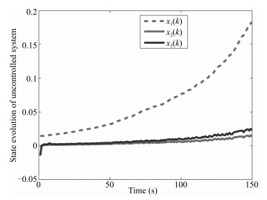 图 2 State evolution $x(k)$ of uncontrolled systems.Fig. 2 State evolution $x(k)$ of uncontrolled systems.
 图 3 State evolution $x(k)$ of controlled systems.Fig. 3 State evolution $x(k)$ of controlled systems.
In order to illustrate the disturbance-attenuation performance, we take the external disturbance
$ \begin{align*} v(k)= \begin{cases} 0.3,&20\leq k\leq 30 \\ -0.2,&50\leq k\leq 60 \\ 0,&\hbox{else}. \end{cases} \end{align*} $
Fig. 4 presents the controller-state evolution $x_c(k)$, Fig. 5 plots the state evolution of the controlled output $z(k)$, and Fig. 6 shows the output feedback controller. From Figs. 3$-$6, one can see that the convergence rate is rapid and effective. By the above simulation results, we can draw the conclusion that our theoretical analysis to the robust $H_\infty$ fuzzy-control problem is right completely.
Remark 2: The above simulation is performed on the basis of the software MATLAB 7.0 and the cone-complementarity linearization algorithm may takes several minutes because of choosing initial feasible set.
6. Conclusion
In this paper, we establish general networked systems model with multiple time-varying random communication delays and multiple missing measurements as weil as the random missing control and discuss its robust $H_\infty$ fuzzy-output feedback-control problem. The proposed system model includes parameter uncertainties, multiple stochastic time-varying delays, multiple missing measurements, and stochastic control input missing. The control strategy adopts the parallel distributed compensation. We obtain the sufficient conditions on the robustly exponential stability of the closed-loop T-S fuzzy-control system by using the CCL algorithm and the explicit expression of the desired controller parameters. An illustrative simulation example further shows that the fuzzy-control method to the proposed new control model is feasible and the new control model can be used for future applications. Whether to construct piecewise Lyapunov functions [8] to solve the proposed control model or not is an interesting topic and in active thought.
-
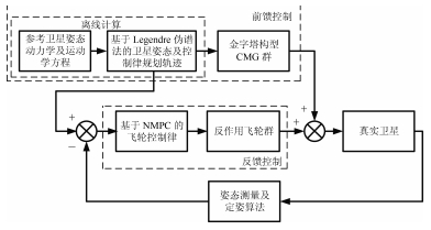
图 4 挠性敏捷卫星姿态控制方案框图
Fig. 4 Diagram of attitude control scheme for flexible agile satellite
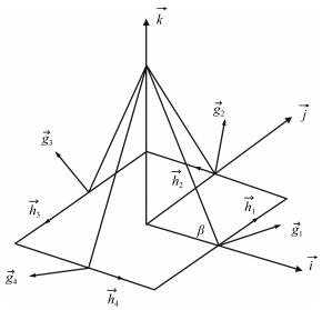
图 5 金字塔构型CMG群系统坐标系示意图
Fig. 5 Diagram of coordinate system for pyramid configuration CMG groups
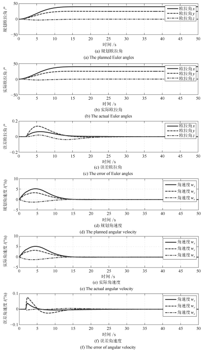
图 6 惯量匹配情况下的姿态大角度机动规划轨迹与实际轨迹曲线对比
Fig. 6 Comparison of planed trajectory and actual trajectory for attitude maneuver in the case of inertia matching
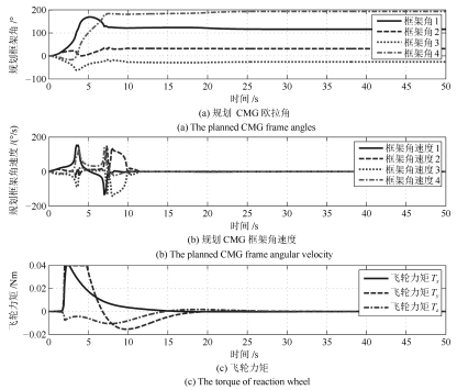
图 7 惯量匹配情况下的规划CMG框架角、角速度与实际飞轮控制力矩曲线
Fig. 7 Planed CMG frame angle, angular velocity and actual flywheel control torque curves in the case of inertia matching
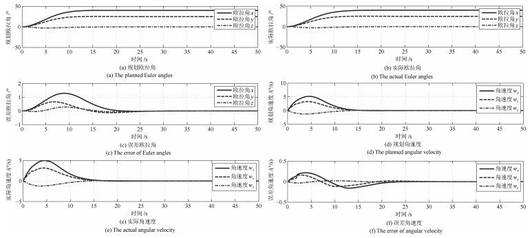
图 8 惯量5 %偏差情况下的姿态大角度机动规划轨迹与实际轨迹曲线对比
Fig. 8 Comparison of planed trajectory and actual trajectory for attitude maneuver with inertia 5 % deviation
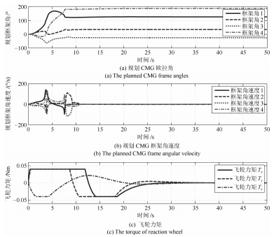
图 9 惯量5 %偏差情况下的规划CMG框架角、角速度与实际飞轮控制力矩曲线
Fig. 9 Planed CMG frame angle, angular velocity and actual flywheel control torque curves with inertia 5 % deviation
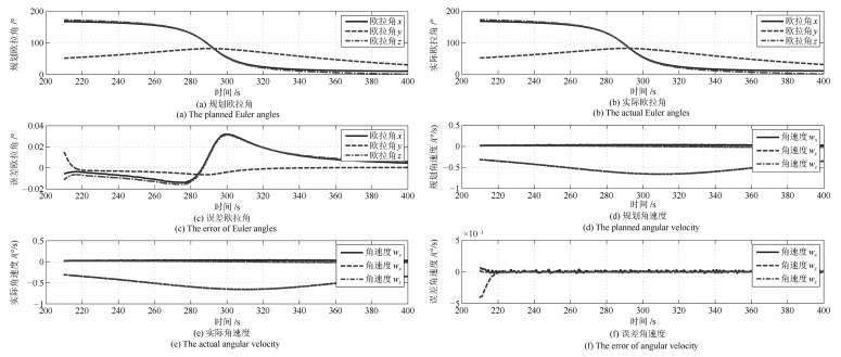
图 10 惯量匹配情况下的凝视成像姿态规划轨迹与实际轨迹曲线对比
Fig. 10 Comparison of planed trajectory and actual trajectory for staring imaging in the case of inertia matching
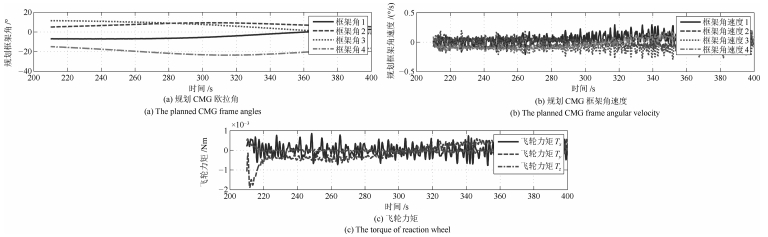
图 11 惯量匹配情况下的规划CMG框架角、角速度与实际飞轮控制力矩曲线
Fig. 11 Planed CMG frame angle, angular velocity and actual flywheel control torque curves in the case of inertia matching
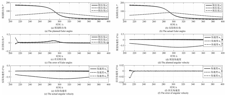
图 12 惯量10 %偏差情况下的凝视成像姿态规划轨迹与实际轨迹曲线对比
Fig. 12 Comparison of planed trajectory and actual trajectory for staring imaging with inertia 10 % deviation
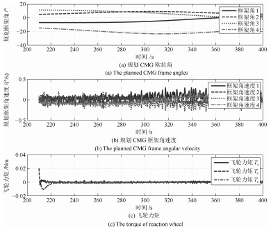
图 13 惯量10 %偏差情况下的规划CMG框架角、角速度与实际飞轮控制力矩曲线
Fig. 13 Planed CMG frame angle, angular velocity and actual flywheel control torque curves with inertia 10 % deviation
表 1 凝视成像过程中的姿态角及角速度约束
Table 1 Attitude angle and angular velocity constraints in staring imaging
过程约束 时间(s) 欧拉角$x\, (^\circ)$ 角速度$w_x\, (^\circ/\rm{s})$ 欧拉角$y\, (^\circ)$ 角速度$w_y\, (^\circ/\rm{s})$ 欧拉角$z\, (^\circ)$ 角速度$w_z\, (^\circ/\rm{s})$ 约束1 250 160.50 0.0297 66.27 –0.4677 163.00 0.0174 约束2 260 155.91 0.0350 70.75 –0.5141 157.61 0.0137 约束3 270 147.50 0.0377 75.40 –0.5590 148.50 0.0135 约束4 280 130.22 0.0391 79.71 –0.5952 130.40 0.0070 约束5 290 94.33 0.0376 82.07 –0.6304 93.91 0.0073 约束6 300 54.46 0.0380 80.19 –0.6499 53.12 0.0060 约束7 310 33.72 0.0351 75.39 –0.6599 31.53 0.0004 约束8 320 23.99 0.0385 69.64 –0.6493 20.96 –0.0015 约束9 330 18.81 0.0373 63.69 –0.6297 14.91 –0.0075 约束10 340 15.77 0.0326 57.87 –0.5962 11.02 –0.0070  下载: 导出CSV
-
[1] Tao J W, Yu W X. A preliminary study on imaging time difference among bands of WorldView-2 and its potential applications. In:Proceeding of the 2011 IEEE International Geoscience and Remote Sensing Symposium. Vancouver, Canada:IEEE, 2011. 198-200 [2] Leeghim H, Lee I H, Lee D H, Bang H, Park J O. Singularity avoidance of control moment gyros by predicted singularity robustness:ground experiment. IEEE Transactions on Control Systems Technology, 2009, 17(4):884-891 doi: 10.1109/TCST.2008.2011556 [3] 李传江, 郭延宁, 马广富.单框架控制力矩陀螺的奇异分析及操纵律设计.宇航学报, 2010, 31(10):2346-2453 doi: 10.3873/j.issn.1000-1328.2010.10.018Li Chuan-Jiang, Guo Yan-Ning, Ma Guang-Fu. Singularity analysis and steering law design for single-gimbal control moment gyroscopes. Journal of Astronautics, 2010, 31(10):2346-2453 doi: 10.3873/j.issn.1000-1328.2010.10.018 [4] 孙志远, 金光, 徐开, 张刘, 杨秀彬.基于力矩输出能力最优的SGCMG操纵律设计.空间科学学报, 2012, 32(1):113-122 doi: 10.11728/cjss2012.01.113Sun Zhi-Yuan, Jin-Guang, Xu Kai, Zhang Liu, Yang Xiu-Bin. Steering law design for SGCMG based on optimal output torque capability. Chinese Journal of Space Science, 2012, 32(1):113-122 doi: 10.11728/cjss2012.01.113 [5] Huntington G T. Advancement and analysis of a gauss pseudospectral transcription for optimal control[Ph. D. dissertation], Massachusetts Institute of Technology, USA, 2007. [6] 杨希祥, 张为华.基于Gauss伪谱法的固体运载火箭上升段轨迹快速优化研究.宇航学报, 2011, 32(1):15-21 http://www.cnki.com.cn/Article/CJFDTOTAL-YHXB201101004.htmYang Xi-Xiang, Zhang Wei-Hua. Rapid optimization of ascent trajectory for solid launch vehicles based on Gauss pseudospectral method. Journal of Astronautics, 2011, 32(1):15-21 http://www.cnki.com.cn/Article/CJFDTOTAL-YHXB201101004.htm [7] Sun C C, Wu S M, Chung H Y, Chang W J. Design of takagi-sugeno fuzzy region controller based on rule reduction, robust control, and switching concept. Journal of Dynamic Systems, Measurement, and Control, 2007, 129(2):163-170 doi: 10.1115/1.2431811 [8] 黄静, 李传江, 马广富, 刘刚.基于广义逆的欠驱动航天器姿态机动控制.自动化学报, 2013, 39(3):285-292 http://www.aas.net.cn/CN/abstract/abstract17802.shtmlHuang Jing, Li Chuan-Jiang, Ma Guang-Fu, Liu Gang. Generalised inversion based maneuver attitude control for underactuated spacecraft. Acta Automatica Sinica, 2013, 39(3):285-292 http://www.aas.net.cn/CN/abstract/abstract17802.shtml [9] 陈刚, 康兴无, 乔洋, 陈士橹.航天器相对大角度姿态跟踪非线性控制器设计.宇航学报, 2009, 32(2):556-559 http://www.cnki.com.cn/Article/CJFDTOTAL-YHXB200902032.htmChen Gang, Kang Xing-Wu, Qiao Yang, Chen Shi-Lu. The nonlinear controller designing for spacecraft large angle attitude state tracking. Journal of Astronautics, 2009, 32(2):556-559 http://www.cnki.com.cn/Article/CJFDTOTAL-YHXB200902032.htm [10] Dong C Y, Xu L J, Chen Y, Wang Q. Networked flexible spacecraft attitude maneuver based on adaptive fuzzy sliding mode control. Acta Astronautica, 2009, 65(11-12):1561-1570 doi: 10.1016/j.actaastro.2009.04.004 [11] Hu Q L, Cao J, Zhang Y Z. Robust backstepping sliding mode attitude tracking and vibration damping of flexible spacecraft with actuator dynamics. Journal of Aerospace Engineering, 2009, 22(2):139-152 doi: 10.1061/(ASCE)0893-1321(2009)22:2(139) [12] Yu S Y, Reble M, Chen H, Allgöwer F. Inherent robustness properties of quasi-infinite horizon nonlinear model predictive control. Automatica, 2014, 50(9):2269-2280 doi: 10.1016/j.automatica.2014.07.014 [13] 常琳, 金光, 范国伟, 徐开.基于terminal滑模控制的小卫星机动方法.光学精密工程, 2015, 23(2):485-496 http://www.cnki.com.cn/Article/CJFDTOTAL-GXJM201502023.htmChang Lin, Jin Guang, Fan Guo-Wei, Xu Kai. Small satellite maneuver based on terminal sliding mode control. Optics and Precision Engineering, 2015, 23(2):485-496 http://www.cnki.com.cn/Article/CJFDTOTAL-GXJM201502023.htm [14] Bernardini D, Bemporad A. Stabilizing model predictive control of stochastic constrained linear systems. IEEE Transactions on Automatic Control, 2012, 57(6):1468-1480 doi: 10.1109/TAC.2011.2176429 [15] Cannon M, Kouvaritakis B, Wu X J. Model predictive control for systems with stochastic multiplicative uncertainty and probabilistic constraints. Automatica, 2009, 45(1):167-172 doi: 10.1016/j.automatica.2008.06.017 [16] 范国伟, 常琳, 戴路, 徐开, 杨秀彬.敏捷卫星姿态机动的非线性模型预测控制.光学精密工程, 2015, 23(8):2318-2327 http://youxian.cnki.com.cn/yxdetail.aspx?filename=MOTO20170110007&dbname=CAPJ2015Fan Guo-Wei, Chang Lin, Dai Lu, Xu Kai, Yang Xiu-Bin. Nonlinear model predictive control of agile satellite attitude maneuver. Optics and Precision Engineering, 2015, 23(8):2318-2327 http://youxian.cnki.com.cn/yxdetail.aspx?filename=MOTO20170110007&dbname=CAPJ2015 [17] 孙光, 霍伟.卫星姿态直接自适应模糊预测控制.自动化学报, 2010, 36(8):1151-1159 http://www.aas.net.cn/CN/abstract/abstract17314.shtmlSun Guang, Huo Wei. Direct-adaptive fuzzy predictive control of satellite attitude. Acta Automatica Sinica, 2010, 36(8):1151-1159 http://www.aas.net.cn/CN/abstract/abstract17314.shtml 期刊类型引用(4)
1. 练红海,肖伸平,罗毅平,周笔锋. 基于T-S模糊模型的采样系统鲁棒耗散控制. 自动化学报. 2022(11): 2852-2862 .  本站查看
本站查看2. 顾晓清,倪彤光,张聪,戴臣超,王洪元. 结构辨识和参数优化协同学习的概率TSK模糊系统. 自动化学报. 2021(02): 349-362 . 本站查看3. 李军,黄卫剑,万文军,刘哲. 一种新型反馈控制器的研究与应用. 控制理论与应用. 2020(02): 411-422 . 百度学术4. 唐晓铭,邓梨,虞继敏,屈洪春. 基于区间二型T-S模糊模型的网络控制系统的输出反馈预测控制. 自动化学报. 2019(03): 604-616 . 本站查看其他类型引用(1)
-

 下载:
下载:


计量
- 文章访问数: 2462
- HTML全文浏览量: 278
- PDF下载量: 510
- 被引次数: 5
