

-
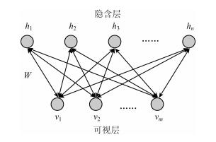
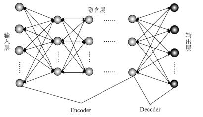
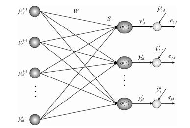
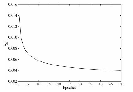
摘要: 针对深度信念网(Deep belief network,DBN)预训练耗时长的问题,提出了一种基于自适应学习率的DBN(Adaptive learning rate DBN,ALRDBN).ALRDBN将自适应学习率引入到对比差度(Contrastive divergence,CD)算法中,通过自动调整学习步长来提高CD算法的收敛速度.然后设计基于自适应学习率的权值训练方法,通过网络性能分析给出学习率变化系数的范围.最后,通过一系列的实验对所设计的ALRDBN进行测试,仿真实验结果表明,ALRDBN的收敛速度得到了提高且预测精度也有所改善.Abstract: A deep belief network with adaptive learning rate (ALRDBN) is proposed to solve the time-consuming problem in the pre-training period of DBN. The ALRDBN introduces the idea of adaptive learning rate into contrastive divergence (CD) algorithm and accelerates its convergence by a self-adjusting learning rate. The training method of weights in this case is designed, in which the adjusting scope of the coefficient in learning rate is determined by performance analysis. Finally, a series of experiments are carried out to test the performance of ALRDBN, and the corresponding results show that the convergence rate is accelerated significantly and the accuracy of prediction is improved as well.
-
1. Introduction
Since recent few decades, some researchers focus their energy on the robust stability and controller design problems about the networked-control systems (NCSs) with some uncertain parameters because some networked-control systems have been succeeded in applications in modern complicated industry processes, e.g., aircraft and space shuttle, nuclear power stations, high-performance automobiles, etc. The fuzzy-logic control based on the Takagi-Sugeno (T-S) is widely used to dealing with complex nonlinear systems because it has simple dynamic structure and highly accurate approximation to any smooth nonlinear function in any compact set. One can consult [1]$-$[8] and the other cited literature therein [9]$-$[31]. Data-packet dropout is an important issue to be addressed in the networked-control systems [6], [32]. Zhang [33] solves the problem of $H_\infty$ estimation for a class of Markov jump linear systems but he neglect possible dropout in practice. Reference [34] reports the problem of $H_\infty$ stability of discrete-time switched linear system with average dwell time and with no dropout. In [6], piecewise Lyapunov function is proposed to analyze robust of the nonlinear NCSs without time-delay issue. Random data-packet dropout and time delay are well considered but the controlled NCSs are linear systems in [32]. Reference [8] discusses the problem of robust $H_\infty$ output feedback control for a class of continuous-time Takagi-Sugeno (T-S) fuzzy affine dynamic systems with parametric uncertainties and input constraints on ignoring some nonlinearities induced by system with data-packet dropout and random time delay. Reference [5] investigates the robust $H_\infty$ stability of a class of half nonlinear NCSs with multiple probabilistic delays and multiple missing measurements regardless of the dropout in the forward path. According to above consideration, we investigate a class of new nonlinear NCSs, in which not only sensors communicate with controllers by network but also controllers do with actuator in the same manner.
The highlights of this paper, which lie primarily on the new research problems and new system models, are summarized as follows:
1) A new model is established, in which the controllers communicate with the actuator by a wireless network and the random missing control from the controller to the actuator occurs and the sensors do with the controllers in the same manner.
2) The investigation on the T-S fuzzy model is used for a class of complex systems that describe the modeling errors, disturbance rejection attenuation, probabilistic delay, missing measurements and missing control within the same framework.
The rest of this paper is organized as follows. The problem under consideration is formulated in Section 2. Development of robust $H_{\infty}$ fuzzy control performance on the exponentially stability the closed-loop fuzzy system are placed in Section 3. Section 4 gives design of robust $H_\infty$ fuzzy controller. An illustrative example is given in Section 5, and we conclude the paper in Section 6.
Notation 1: The notation used in the paper is fairly standard. %The superscript "T" stands for matrix transpose; $\mathbb{R}^n$ denotes the $n$-dimensional real vectors; $\mathbb{R}^{m\times n}$ denotes the $n$-dimensional matrix; and $I$ and 0 represent the identity matrix and zero matrix, respectively. The notation $P>0$ ($P\geq 0$) means that $P$ is real symmetric and positive definite (semi-definite), ${\rm tr}(M)$ refers to the trace of the matrix $M$, and $ \|\cdot\|_2 $ stands for the usual $l_2$ norm. In symmetric block matrices or complex matrix expressions, we use an "$\star$" to represent a term that is induced by symmetry, and ${\rm diag}\{\cdots\}$ stands for a block-diagonal matrix. In addition, ${E}\{x\}$ and ${E}\{x|y\}$ will, respectively, mean expectation of $x$ and expectation of $x $ conditional on $y$.
2. Problem Formulation
In this note, the output feedback control problem for discrete-time fuzzy systems in NCSs is taken in our consideration, where the frame-work is depicted in Fig. 1.
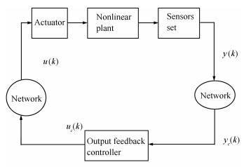 图 1 Framework of output feedback control systems over network environment.Fig. 1 Framework of output feedback control systems over network environment.
The sensors are connected to a network, which are shared by other NCSs and susceptible to communication delays and missing measurements or pack dropouts). As Fig. 1 depicts, pack dropouts from the controller to actuator can take place stochastically. The fuzzy systems with multiple stochastic communication delays and uncertain parameters can be read as follows:
Plant Rule $i$: If $\theta_{1}(k) $ is $ M_{i1}$, and $\theta_{2}(k)$ is $M_{i2}$, and, $\ldots$, and $\theta_{p}(k)$ is $M_{ip}$, then
$ \begin{align} x(k+1)=&\ A_i(k)x(k)+A_{di}\sum\limits_{m=1}^{h}\alpha_m(k)x(k-\tau_m(k))\notag\\ & +B_{1i}u(k)+D_{1i}v(k)\notag\\ \tilde{y}(k)=&\ C_ix(k)+D_{1i}v(k)\notag\\ z(k)=&\ C_{zi}(k)+B_{2i}u(k)+D_{3i}v(k)\notag\\ x(k)=&\ \phi(k)\quad\forall\, {k}\in \mathbb{Z}^{-}, ~\, i=1, \ldots, r \end{align} $
(1) where $M_{ij}$ is the fuzzy set, $r$ stands for the number of If-then rules, and $\theta(k)=[\theta_1(k), \theta_2(k), \ldots, \theta_{p}(k)]$ is the premise variable vector, which is independent of the input variable $u(k)$. $x(k)\in \mathbb{R}^n$ is the state vector, $u(k)\in \mathbb{R}^m$, $\tilde{y}$ $\in$ $\mathbb{R}^s$ is the process output, $z(k)\in \mathbb{R}^q$ is the controlled output, $v(k)\in \mathbb{R}^p$ presents a vector of exogenous inputs, which belongs to $l_2[0, \infty)$, $\tau_m(k)$ $(m=1, 2, \ldots, h)$ are the communication delays that vary with the stochastic variables $\alpha_m(k)$, and $\phi(k)$ $(\forall\, {k}\in \mathbb{Z}^{-})$ is the initial state.
The stochastic variables $\alpha_m(k)\in \mathbb{R}$ $(m=1, 2, \ldots, h)$ in (1) are assumed to satisfy mutually uncorrelated Bernoulli-distributed-white sequences described as follows:
$ \begin{align} & {\rm Prob}\{\alpha_m(k)=1\}={E}\{\alpha_m(k)\}=\bar{\alpha}_m\notag\\ & {\rm Prob}\{\alpha_m(k)=0\}=1-\bar{\alpha}_m.\notag \end{align} $
In this note, one can make the random communication-time delays satisfy the following assumption that the time-varying $\tau_m(k)$ $ (m=1, 2, \ldots, h)$ are subject to $ d_t\leq \tau_m(k)$ $\leq$ $d_T$. The matrices $A_i(k)=A_i+\Delta{A_i(k)}$, $C_{zi}(k)= C_{zi}$ $+$ $\Delta{C_{zi}}(k)$, where $ A_i, A_{di}, B_{1i}, B_{2i}, C_i, C_{zi}, D_{1i}, D_{2i}$, and $D_{3i}$ are known constant matrices with compatible dimensions. $\Delta{A_i(k)} $ and $\Delta C_{zi}(k)$ with the time-varying norm-bounded uncertainties satisfy
$ \begin{align} \left[ \begin{array}{c} \Delta A_i(k)\\ \Delta C_{zi}(k)\\ \end{array} \right]=\left[ \begin{array}{c} H_{ai}\\ H_{ci}\\ \end{array} \right]F(k)E \end{align} $
(2) with $H_{ai}$, $H_{ci}$ being constant matrices and $F^T(k)F(k)\leq I$, $\forall\, {k}$.
In this note, the packet dropout (the miss-measurement) read as
$ \begin{align} y_c(k)&= \Xi{C_i}x(k)+D_{2i}(k)\notag\\ &=\sum\limits_{l=1}^{s}\beta_lC_{il}x(k)+D_{2i}v(k)\notag\\ u(k)&=W(k)u_c(k)=W(k)C_{ki}x_c(k) \end{align} $
(3) where $\Xi=\hbox{diag}\{\beta_1, \ldots, \beta_s\}$ with $\beta_l$ $(l=1, 2, \ldots, s)$ being $s$ unrelated random variables, which are also unrelated with $\alpha_m(k)$ and $W(k)$ denoting the random packet missing from the controllers to the actuator. One can assume that $\beta_l $ has the probabilistic-density function $q_l(s)$ $(l=1, 2, \ldots, s)$ on the interval $[0, 1]$ with mathematical expectation $\mu_l$ and variance $\sigma_l^2$. $C_{il}={\rm diag}\{\underbrace{0, \ldots, 0}\limits_{l-1}, 1, \underbrace{0, \ldots, 0}\limits_{s-l}\}C_i$. We denote the stochastic pack dropouts from the controller to the actuator by $W(k)= {\rm diag}\{\omega_1(k), \ldots, \omega_m(k)\}$, where $\omega_l$ $(l=$ $1, 2, \ldots, m)$ are mutually unrelated random variables and obey Bernoulli distribution with mathematical expectation $\bar{\omega}_l$ and variance$\rho_l $and assumed to be unrelated with $\alpha_m(k)$. For a given pair of $(x(k), u(k))$, the final output of the fuzzy system is read as
$ \begin{align} x(k+1)=&\, \sum\limits_{i=1}^{r}h_i(\theta(k))[A_i(k)x(k)+B_{1, i}u(k)\notag\\ &\, +A_{di}\sum\limits_{m=1}^{h}x(k-\tau_m(k))+D_{1i}v(k)]\notag\\ y_c(k)=&\, \sum\limits_{i=1}^{r}h_i(\theta(k))[\Xi{C_i}x(k)+D_{2i}v(k)]\notag\\ z(k)=&\, \sum\limits_{i=1}^{r}h_i(\theta(k))[C_{zi}(k)x(k)+B_{2i}u(k)+D_{3i}v(k)] \end{align} $
(4) where the fuzzy-basis functions are described as
$ \begin{align} &{h_i(\theta(k))}=\frac {\vartheta_i(\theta(k))} {\sum\limits_{i=1}^{r}\vartheta_i(\theta(k))}\notag\\ &\vartheta_i(\theta(k))=\prod\limits_{j=1}^{p}M_{ij}(\theta_j(k))\notag \end{align} $
with $M_{ij}(\theta_j(k))$ being the grade of membership of $\theta_j(k)$ in $M_{ij}$. It is clear that $\vartheta_i(\theta(k))\geq 0$, $i=1, 2, \ldots, r$, $\sum_{i=1}^{r}\vartheta_i(\theta(k))>0$, $\forall\, {k}$, and $h_i(\theta(k))\geq 0$, $i=1, 2, \ldots, r$, $\sum_{i=1}^{r}h_i(\theta(k))=1$, $\forall\, {k}$. In the sequel, we denote $h_i=h_i(\theta(k))$ for brevity.
In the note, the fuzzy dynamic output-feedback controller for the fuzzy system (4) is given as
Controller Rule $i$: If $\theta_1(k)$ is $M_{il}$ and $\theta_2(k)$ is $M_{i2}$ and, $\ldots$, and $\theta_p(k)$ is $M_{ip}$ then
$ \begin{align} \begin{cases} x_c(k+1)=A_{ki}x_c(k)+B_{ki}y_c(k)\\ u(k)= W(k)C_{ki}x_c(k) \end{cases} \end{align} $
(5) with $x_c(k)\in \mathbb{R}^n$ being the controller state along with the controller parameters $A_{ki}$, $B_{ki}$ and $C_{ki}$ to be determined. Naturally, the overall fuzzy output-feedback controller is read as
$ \begin{align} \begin{cases} x_c(k+1)=\sum\limits_{i=1}^{r}h_i[A_{ki}x_c(k)+B_{ki}y(k)]\\ u(k)=\sum\limits_{i=1}^{r}h_iW(k)C_{ki}x_c(k), \ \ i=1, 2, \ldots, r. \end{cases} \end{align} $
(6) Combining (6) with (4), we can obtain the closed-loop system described as
$ \begin{align} \begin{cases} \bar{x}(k+1)=\sum\limits_{i-1}^{r}\sum\limits_{j=1}^{r}h_ih_j[(A_{ij}+B_{ij})\bar{x}(k)+D_{ij}v(k) \\ \qquad \qquad \quad\, +\sum\limits_{m=1}^{h}(\bar{A}_{dmi}+\tilde{A}_{dmi})\bar{x}(k-\tau_m(k)]\\ z(k)=\sum\limits_{i=1}^{r}\sum\limits_{j=1}^{r}h_ih_j[\bar{C}_{ij}(k)+\bar{\bar{C}}_{ij}]\bar{x}(k) +D_{3i}v(k) \end{cases} \end{align} $
(7) where
$ \begin{align*} &\bar{x}(k)=\left[ \begin{array}{c} x(k) \\ x_c(k) \\ \end{array} \right], \quad A_{ij}=\left[ \begin{array}{cc} A_i(k)&B_{1i}\bar{W}C_{kj} \\ B_{ki}\bar{\Xi}C_j&A_{ki} \\ \end{array} \right]\\[1mm] &B_{ij}=\left[ \begin{array}{cc} 0& B_{1i}\tilde{W}(k)C_{kj}\\ B_{ki}\tilde{\Xi}C_j& 0\\ \end{array} \right]\\[1mm] &\bar{A}_{dmi}=\left[ \begin{array}{cc} \bar{\alpha}_mA_{di}&0 \\ 0&0 \\ \end{array} \right], \quad \tilde{A}_{dmi}=\left[ \begin{array}{cc} \tilde{\alpha}_mA_{di}&0 \\ 0&0 \\ \end{array} \right]\\[1mm] &D_{ij}=\left[ \begin{array}{c} D_{1i} \\ B_{ki}D_{2j} \\ \end{array} \right], \quad \bar{C}_{ij}(k)=\bigg[ \begin{array}{cc} C_{zi}(k)&B_{2i}\bar{W}C_{kj} \\ \end{array} \bigg]\\[1mm] &\bar{\bar{C}}_{ij}(k)=\bigg[ \begin{array}{cc} 0&B_{2i}\tilde{W}(k)C_{kj} \\ \end{array} \bigg] \end{align*} $
with $\tilde{\alpha}_m(k)=\alpha_m(k)-\bar{\alpha}_m(k)$ and $\tilde{\omega}_j(k)={\omega}_j(k)-\bar{\omega}_j(k)$. It is evident that $E\{\tilde{\alpha}_m(k)\}=0$ and that $E\{\tilde{\omega}_j(k)\}=0$ and that $E\{\tilde{\alpha}_m^2(k)\}=\bar{\alpha}_m(1-\bar{\alpha}_m)=\sigma_m^2$ and that $E\{\tilde{\omega}_j^2(k)\}$ $=$ $\bar{\omega}_j(1-\bar{\omega}_j)=\rho_j^2$.
Denote
$ \begin{align*} &\bar{x}(k-\tau)\\ &=\left[ \!\!\begin{array}{cccc} \ \ \bar{x}^T(k-\tau_1(k)) &\!\bar{x}^T(k-\tau_2(k))&\! \cdots &\!\bar{x}^T(k-\tau_h(k))\ \ \\ \end{array} \!\!\right]^T\\ &\xi(k)=\left[ \begin{array}{ccc} \bar{x}^T(k)&\bar{x}^T(k-\tau) &v^T(k) \\ \end{array} \right]^T\end{align*} $
then (7) can also be rewritten as
$ \begin{align} \begin{cases} \bar{x}(k+1) =\sum\limits_{i=1}^{r}\sum\limits_{j=1}^{r}h_ih_j\left[A_{ij}\!+B_{ij}, \hat{Z}_{mi}\!+\Delta\hat{Z}_{mi}, D_{ij}\right]\xi(k) \\ z(k)=\sum\limits_{i=1}^{r}\sum\limits_{j=1}^{r}h_ih_j\left[\bar{C}_{ij}+ \bar{\bar{C}}_{ij}, 0, D_{3i}\right]\xi(k) \end{cases} \end{align} $
(8) where $\hat{Z}_{mi}=[\bar{A}_{d1i}, \ldots, \bar{A}_{dhi}]$ and $\Delta\hat{Z}_{mi}=[\tilde{A}_{d1i}, \ldots, \tilde{A}_{dhi}]$. In order to smoothly formulate the problem in the note, we introduce the following definition.
Definition 1: For the system (7) and every initial conditions $\phi$, the trivial solution is said to be exponentially mean square stable if, in the case of $v(k)=0$, there exist constants $\delta>0$ and $0<\kappa<1$ such that $E\{\|\bar{x}(k)\|^2\}$ $\leq$ $\delta\kappa^k \sup_{-d_M\leq i\leq 0}E\{\|{\phi(i)}\|^2\}$, $\forall\, {k}\geq 0$.
We will develop techniques to settle the robust $H_{\infty}$ dynamic output feedback problem for the discrete-time fuzzy system (7) subject to the following conditions:
1) The fuzzy system (7) is exponentially stable in the mean square.
2) Under zero-initial condition, the controlled output $z(k)$ satisfies
$ \begin{align} \sum\limits_{k=0}^{\infty}E\left\{\|{z(k)}\|^2\right\}\leq \gamma^2\sum\limits_{k=0}^{\infty}E\left\{\|{v(k)}\|^2\right\} \end{align} $
(9) for all nonzero $v(k)$, where $\gamma>0$ is a prescribed scalar.
Remark 1: The proposed new model has the function that not only the controllers communicate with the actuator by wireless but also the sensors do with the controllers by the same manner.
3. Development of Robust ${\pmb H}_{\pmb \infty}$ Fuzzy Control Performance
At first, we give the following lemma, which will be adopted in obtaining our main results.
Lemma 1 (Schur complement): Given constant matrices $S_1$, $S_2$, $S_3$, where $S_1=S_1^T$ and $0<S_2=S_2^T$, then $ S_1$ $+$ $S_3^TS_2^{-1}S_3$ $<$ $0$ if and only if
$ \begin{align*} \left[ \begin{array}{cc} S_1&S_3^T \\ S_3 &-S_2 \\ \end{array} \right]<0~~ \hbox{or}~~ \left[ \begin{array}{cc} -S_2&S_3 \\ S_3^T&S_1 \\ \end{array} \right]<0. \end{align*} $
Lemma 2 (S-procedure) [5]: Letting $L=L^T$ and $H$ and $E$ be real matrices of appropriate dimensions with $F$ satisfying $FF^T\leq I$, then $ L+HFE+E^TF^TH^T<0$ if and only if there exists a positive scalar $\varepsilon>0$ such that $L$ $+$ $\varepsilon^{-1}HH^T+\varepsilon E^TE<0$, or equivalently
$ \begin{align*} \left[ \begin{array}{ccc} L&H&\varepsilon{E^T} \\ H^T &-\varepsilon{I}&0 \\ \varepsilon{E}&0 &-\varepsilon{I} \\ \end{array} \right]<0. \end{align*} $
Lemma 3: For any real matrices $X_{ij}$ for $i$, $j=1, 2, \ldots, $ $r$ and $n>0$ with appropriate dimensions, we have [35]
$ \sum\limits_{i=1}^r\sum\limits_{j=1}^r\sum\limits_{l=1}^r\sum\limits_{l=1}^rh_ih_jh_kh_lX_{ij}^T\Lambda{X_{kl}}\leq\sum\limits_{i=1}^r\sum\limits_{j=1}^rh_ih_jX_{ij}^T\Lambda X_{ij}. $
Theorem 1: For given controller parameters and a prescribed $H_{\infty}$ performance $\gamma>0$, the nominal fuzzy system (7) is exponentially stable if there exist matrices $P>0$ and $Q_k$ $>$ $0$, $k=1, 2, \ldots, h$, satisfying
$ \left[ \begin{array}{cc} \Pi_i&\star \\ 0.5\Sigma_{ii}&\bigwedge \\ \end{array} \right]<0 $
(10) $ \left[ \begin{array}{cc} 4\Pi_i&\star \\ \Sigma_{ij}&\bigwedge \\ \end{array} \right]<0, \quad 1\leq i<j\leq r $
(11) where
$ \Pi_i =\ {\rm diag}\bigg\{-P+\sum\limits_{k=1}^h(d_T-d_t+1)Q_k, \hat{\alpha}\breve{A}_{di}^T\breve{P} \breve{A}_{di}\notag\\ \ \ \ \ \ \ -{\rm diag}\{Q_1, Q_2, \ldots, Q_h\}, -\gamma^2I\bigg\} $
(12) $\begin{align*} \hat{\alpha}=&\ {\rm diag}\left\{\bar{\alpha}_1(1-\bar{\alpha}_1), \ldots, \bar{\alpha}_h(1-\bar{\alpha}_h)\right\}\notag\\ \breve{A}_{di}=&\ {\rm diag}\{\underbrace{\hat{A}_{di}, \ldots, \hat{A}_{di}}\limits_h\}\notag\\ \check{C}_{ij}=&\ \left[\sigma_1\hat{C}_{11ij}^TP, \ldots\!, \sigma_s\hat{C}_{1sij}^TP, \rho_1\hat{C}_{k1ij}^TP, \ldots\!, \rho_m\hat{C}_{kmij}^TP\right]^T\notag\\ &\check{P}=\hbox{diag}\{\underbrace{P, \ldots, P}\limits_{s+m}\}\\ &{\small\bigwedge}=\hbox{diag}\{-\check{P}, -P, -I, \hbox{diag}\{\underbrace{-I, \ldots, -I}\limits_m\}\}\\ &\breve{P}=\hbox{diag}\{\underbrace{P, \ldots, P}\limits_h\}\\ &\hat{A}_{di}=\left[ \begin{array}{cc} A_{di}&0\\ 0&0\\ \end{array} \right] \\ &\Sigma_{ij}=\\ &\!\!\!\left[\!\!{\small \begin{array}{ccccc} \check{C}_{ij}\!+\!\check{C}_{ji}\! &\! 0\!&\!0 \\[2mm] PA_{ij}\!+\!PA_{ji} \! &\! P\hat{Z}_{mi}\!+\!P\hat{Z}_{mj} \! &\!PD_{ij}\!+\!PD_{ji}\\[2mm] \bar{C}_{ij}\!+\!\bar{C}_{ji}\! &\!0\! &\!D_{3i}\!+\!D_{3j}\\[2mm] \, [0 ~~ \rho_1B_{2i}C_{kj1}\!+\!\rho_1B_{2j}C_{ki1}] \! &\!0\! &\!0\\[2mm] \vdots\! &\!\vdots\! &\!\vdots\\[2mm] \, [0 ~~ \rho_mB_{2i}C_{kjm}\!+\!\rho_mB_{2j}C_{kim}]\! &\!0\! &\!0\\ \end{array}}\!\!\!\! \right]. \end{align*} $
Proof:
Let
$ \begin{align*} &\Theta_j(k)=\{x(k-\tau_j(k), x(k-\tau_j(k)+1, \ldots, x(k)\}\\ &\chi(k)=\{\Theta_1(k)\bigcup\Theta_2(k)\bigcup\ldots\bigcup\Theta_h(k)\}=\bigcup\limits_{j=1}^{h}\Theta_j(k) \end{align*} $
where $j=1, 2, \ldots, h$. We consider the following Lyapunov functional for the system of (7): $V(\chi(k))=\sum_{i=1}^3V_i(k)$, where
$ \begin{align*} &V_1(k)=\bar{x}^T(k)P\bar{x}\\ &V_2(k)=\sum\limits_{j=1}^{h}\sum\limits_{i=k-\tau_j(k)}^{k-1}\bar{x}^T(i)Q_j\bar{x}(i)\\ &V_3(k)=\sum\limits_{j=1}^h\sum\limits_{m=-d_M+1}^{-d_m}\sum\limits_{i=k+m}^{k-1}\bar{x}^T(i)Q_j\bar{x}(i) \end{align*} $
with $P>0$, $Q_j>0$ $(j=1, 2, \ldots, h)$ being matrices to be determined.
$ \begin{align} {E}[\Delta{V}|x(k)]&={E}[V(\chi(k+1))|\chi(k)]-V(\chi(k))\notag\\ & ={E}[(V(\chi(k+1))-V(\chi(k)))|\chi(k)]\notag\\ & =\sum\limits_{i=1}^{3}{E}[\Delta{V_i}|\chi(k)]. \end{align} $
(13) According to (7), we have
$ \begin{align*} &{E}\{\Delta{V_1}|\chi(k)\}\\ &\qquad={E} \left[(\bar{x}^T(k+1)P\bar{x}(k+1)-\bar{x}^T(k)P\bar{x}(k))|\chi(k)\right]\\ &\qquad\leq\xi^T(k)\sum\limits_{i=1}^{r}\sum\limits_{j=1}^{r}\Omega_{ij}\xi(k) \end{align*} $
where
$ \begin{align} & {{\Omega }_{ij}}=E\left\{ \left[\begin{matrix} A_{ij}^{T}P{{A}_{ij}}+B_{ij}^{T}P{{B}_{ij}}-P & {} \\ \star & {} \\ \star & {} \\ \end{matrix} \right. \right. \\ & \left. \left. \begin{matrix} {} & A_{ij}^{T}P{{{\hat{Z}}}_{mi}} & A_{ij}^{T}P{{D}_{ij}} \\ {} & \hat{Z}_{mi}^{T}P{{{\hat{Z}}}_{mi}}+\Delta \hat{Z}_{mi}^{T}P\Delta {{{\hat{Z}}}_{mi}} & \hat{Z}_{mi}^{T}P{{D}_{ij}} \\ {} & \star & D_{ij}^{T}P{{D}_{ij}} \\ \end{matrix} \right] \right\} \\ \end{align} $
$ {{B}_{ij}}=\left[\begin{matrix} 0 & 0 \\ {{B}_{ki}}\tilde{\Xi }{{C}_{j}} & 0 \\ \end{matrix} \right]+\left[\begin{matrix} 0 & {{B}_{1i}}\tilde{\omega }(k){{C}_{kj}} \\ 0 & 0 \\ \end{matrix} \right] $
$ \begin{align} & E\{B_{ij}^{T}P{{B}_{ij}}\} \\ & \ \ \ \ \ =\sum\limits_{l=1}^{s}{\sigma _{l}^{2}}{{\left[\begin{matrix} 0 & 0 \\ {{B}_{ki}}{{C}_{jl}} & 0 \\ \end{matrix} \right]}^{T}}P\left[\begin{matrix} 0 & 0 \\ {{B}_{ki}}{{C}_{jl}} & 0 \\ \end{matrix} \right] \\ & \ \ \ \ \ +\sum\limits_{l=1}^{m}{\rho _{l}^{2}}{{\left[\begin{matrix} 0 & {{B}_{1i}}{{C}_{kjl}} \\ 0 & 0 \\ \end{matrix} \right]}^{T}}P\left[\begin{matrix} 0 & {{B}_{1i}}{{C}_{kjl}} \\ 0 & 0 \\ \end{matrix} \right] \\ & \ \ \ ={{({{{\overset{\lower0.5em\hbox{$\smash{\scriptscriptstyle\smile}$}}{P}}}^{-1}}{{{\overset{\lower0.5em\hbox{$\smash{\scriptscriptstyle\smile}$}}{C}}}_{lij}})}^{T}}\overset{\lower0.5em\hbox{$\smash{\scriptscriptstyle\smile}$}}{P}({{{\overset{\lower0.5em\hbox{$\smash{\scriptscriptstyle\smile}$}}{P}}}^{-1}}{{{\overset{\lower0.5em\hbox{$\smash{\scriptscriptstyle\smile}$}}{C}}}_{lij}}) \\ \end{align} $
$ \begin{align} & \overset{\lower0.5em\hbox{$\smash{\scriptscriptstyle\smile}$}}{P}=\rm{diag}\{\underbrace{\mathit{P}, \ldots, \mathit{P}}_{\mathit{s}+\mathit{m}}\} \\ & {{{\hat{C}}}_{1lij}}=\left[\begin{matrix} 0 & 0 \\ {{B}_{ki}}{{C}_{jl}} & 0 \\ \end{matrix} \right] \\ & {{{\hat{C}}}_{klij}}=\left[\begin{matrix} 0 & {{B}_{1i}}{{C}_{kjl}} \\ 0 & 0 \\ \end{matrix} \right] \\ & {{{\overset{\lower0.5em\hbox{$\smash{\scriptscriptstyle\smile}$}}{C}}}_{ij}}={{\left[{{\sigma }_{1}}\hat{C}_{11ij}^{T}P, \ldots, {{\sigma }_{s}}\hat{C}_{1sij}^{T}P, {{\rho }_{1}}\hat{C}_{k1ij}^{T}P, \ldots, {{\rho }_{m}}\hat{C}_{kmij}^{T}P \right]}^{T}} \\ \end{align} $
$ \begin{align} & E\left\{ \Delta \hat{Z}_{mi}^{T}P\Delta {{{\hat{Z}}}_{mi}} \right\} \\ & \ \ \ \ \ =\sum\limits_{m=1}^{h}{{{{\bar{\alpha }}}_{m}}}(1-{{{\bar{\alpha }}}_{m}}){{\left[ \begin{matrix} {{A}_{di}} & 0 \\ 0 & 0 \\ \end{matrix} \right]}^{T}}P\left[ \begin{matrix} {{A}_{di}} & 0 \\ 0 & 0 \\ \end{matrix} \right] \\ & \ \ \ \ \ \ =\sum\limits_{m=1}^{h}{\hat{A}_{di}^{T}}P{{{\hat{A}}}_{di}}=\hat{\alpha }\overset{\lower0.5em\hbox{$\smash{\scriptscriptstyle\smile}$}}{A}_{di}^{T}\overset{\lower0.5em\hbox{$\smash{\scriptscriptstyle\smile}$}}{P}{{{\overset{\lower0.5em\hbox{$\smash{\scriptscriptstyle\smile}$}}{A}}}_{di}} \\ \end{align} $
$ \begin{align} & \hat{\alpha }=\rm{diag}\{{{{\bar{\alpha }}}_{1}}(1-{{{\bar{\alpha }}}_{1}}), \ldots, {{{\bar{\alpha }}}_\mathit{h}}(1-{{{\bar{\alpha }}}_\mathit{h}})\} \\ & {{{\overset{\lower0.5em\hbox{$\smash{\scriptscriptstyle\smile}$}}{A}}}_{di}}=\rm{diag}\{\underbrace{\mathit{{{\hat{A}}}_{di}}, \ldots, \mathit{{{\hat{A}}}_{di}}}_\mathit{h}\} \\ & E\{\Delta {{V}_{2}}|\chi (k)\}\le E\{\sum\limits_{j=1}^{h}{({{{\bar{x}}}^{T}}(}k){{Q}_{j}}\bar{x}(k) \\ & \ \ \ \ \ -{{{\bar{x}}}^{T}}(k-{{\tau }_{j}}(k)){{Q}_{j}}\bar{x}(k-{{\tau }_{j}}(k)) \\ & \ \ \ \ \ +\sum\limits_{i=k-{{d}_{M}}+1}^{k-{{d}_{m}}}{{{{\bar{x}}}^{T}}}(i){{Q}_{j}}\bar{x}(i))|\chi (k)\} \\ & E\{\Delta {{V}_{3}}|\chi (k)\}=E\{\sum\limits_{j=1}^{h}{((}{{d}_{T}}-{{d}_{t}}){{{\bar{x}}}^{T}}(k){{Q}_{j}}\bar{x}(k) \\ & \ \ \ \ \ -\sum\limits_{i=k-{{d}_{m}}+1}^{k-{{d}_{m}}}{{{{\bar{x}}}^{T}}}(i){{Q}_{j}}\bar{x}(i))|\chi (k)\}. \\ \end{align} $
It is clear that
$ {E}\{\Delta{V_2}|\chi(k)\}+{E}\{\Delta{V_3}|\chi(k)\}\leq\xi^T(k)T_{ij}\xi(k) $
with
$ \begin{align*} T_{ij}=&\ \hbox{diag}\Bigg\{\sum\limits_{k=1}^h(d_T-d_t+1)Q_k, \\ &-\hbox{diag}\{Q_1, Q_2, \ldots, Q_h\}, 0\Bigg\}.\end{align*} $
Therefore, we have ${E}\{\Delta{V}|\chi(k)\}\leq\xi^T(k)\Gamma_{ij}\xi(k)$, where $\Gamma_{ij}$ $=$ $\Omega_{ij}+T_{ij}$. Due to
$ \begin{align*} &{E}\left\{z^T(k)z(k)-\gamma^2v^T(k)v(k)\right\}\\ &\qquad\leq\xi(k)\sum\limits_{i=1}^r\sum\limits_{j=1}^rh_ih_j {E}\left\{[\bar{C}_{ij}+\bar{\bar{C}}_{ij}, 0, D_{3i}]^T\right.\\ &\qquad\quad \left.\times[\bar{C}_{ij}+\bar{\bar{C}}_{ij}, 0, D_{3i}] - \hbox{diag}\{0, 0, \gamma^2I\}\right\}\xi(k) \end{align*} $
we can obtain
$ \begin{align*} &{E}\left\{z^T(k)z(k)-\gamma^2v^T(k)v(k)+\Delta{V(k)}\right\}\\ &\qquad \leq\xi^T(k)({\Omega}_{ij}^T\hbox{diag} \{P, I\}{\Omega}_{ij}\\ &\qquad\quad +\mathcal{Z}_{ij}^T\hbox{diag}\{\check{P}, I\}\mathcal{Z}_{ij}+\bar{P})\xi(k) \end{align*} $
where
$ \begin{align*} &{\Omega}_{ij}=\left[ \begin{array}{ccc} A_{ij}&\hat{Z}_{mi}&D_{ij}\\ \bar{C}_{ij}&0&D_{3i}\\ \end{array} \right]\\ & \Game _{kijt}= \bigg[ \begin{array}{ccc} \left[ \begin{array}{cc} 0&\rho_tB_{2i}C_{kjt} \end{array} \right]&0&0 \end{array} \bigg]^T \\ &\mathfrak{D}_{ij}=\bigg[ \begin{array}{ccc} \Game_{kij1}&\ldots&\Game_{kijm} \end{array} \bigg]^T \\ &\mathcal{Z}_{ij}=\left[ \begin{array}{c} [\check{P}^{-1}\check{C}_{ij}, 0, 0]\\ \mathfrak{D}_{ij} \end{array} \right]\\ &\bar{P}=\hbox{diag}\bigg\{-P+\sum\limits_{k=1}^h(d_T-d_t+1)Q_k, \hat{\alpha}\breve{A}_{di}^T\breve{P} \breve{A}_{di}\\ &\qquad -\hbox{diag}\{Q_1, Q_2, \ldots, Q_h\}, -\gamma^2I\bigg\}. \end{align*} $
Define $J(n)={E}\sum\nolimits_{k=0}^n[z^T(k)z(k)-\gamma^2v^T(k)v(k)]$, we have
$ \begin{align*} J(n)=&\ {E}\sum\limits_{k=0}^n\left[z^T(k)z(k)-\gamma^2v^T(k)v(k)+\Delta{V(\chi(k))}\right] \\ &-{E}V(\chi(n+1))\\ \leq&\ {E}\sum\limits_{k=0}^n\left[z^T(k)z(k)-\gamma^2v^T(k)v(k)+\Delta{V(\chi(k))}\right]\\ \leq&\ \sum\limits_{k=0}^n\sum\limits_{i=1}^r\sum\limits_{j=1}^rh_ih_j\xi^T(k)({\Omega}_{ij}^T \hbox{diag} \{P, I\}{\Omega}_{ij}\\ &\ +\mathcal{Z}_{ij}^T\hbox{diag}\{\check{P}, I\}\mathcal{Z}_{ij}+\bar{P})\xi(k)\\ =&\ \sum\limits_{k=0}^n\sum\limits_{i=1}^rh_i^2\xi^T(k)({\Omega}_{ii}^T \hbox{diag} \{P, I\}{\Omega}_{ii}\\ &\ +\mathcal{Z}_{ii}^T\hbox{diag}\{\check{P}, I\}\mathcal{Z}_{ii}+\bar{P})\xi(k)\\ &\ +\frac{1}{2}\sum\limits_{k=0}^n\sum\limits_{j=1, i<j}^rh_ih_j\xi^T(k)\\ &\ \times\left[({\Omega}_{ij} +{\Omega}_{ji})^T\hbox{diag}\{P, I\}({\Omega}_{ij}+{\Omega}_{ji})\right.\\ &\ +\left. (\mathcal{Z}_{ij}+\mathcal{Z}_{ji})^T\hbox{diag}\{\check{P}, I\} (\mathcal{Z}_{ij}+\mathcal{Z}_{ji})+4\bar{P}\right]\xi(k). \end{align*} $
According to Schur complement, we can conclude from (10) and (11) that $J(n)<0$. Letting $n\rightarrow\infty$, we have
$ \begin{align*} \sum\limits_n^\infty{E}\left\{\|z(k)\|^2\right\}\leq\gamma^2\sum\limits_n^\infty{E}\left\{\|v(k)\|^2\right\}. \end{align*} $
According to Schur complement again, we know that ${E}\{\Delta{V}|x(k)\}$ $<$ $0$ if and only if (10) and (11) hold true. Furthermore, one can easily verify the fact that the discrete-time nominal (7) with $v(k)=0$ is exponentially stable.
4. Design of Robust ${\pmb H}_{\pmb\infty}$ Fuzzy Controller
In this section, we are devoted to how to determine the controller parameters in (6) such that the closed-loop system (7) is exponentially stable with $H_\infty$ performace.
By Theorem 1, one can easily draw the conclusion as follow:
Theorem 2: For a prescribed constant $\gamma>0$, the nominal fuzzy system (7) is exponentially stable if there exist positive definite matrices $P>0$, $L>0$, $Q_k>0$ $(k=1, 2, $ $\ldots, $ $h)$, and $K_i$ and $\bar{C}_{ki}$ such that
$ \Gamma_1=\left[ \begin{array}{cc} \Pi_i&\star \\ 0.5\bar{\Sigma}_{ii}& \bar{\Lambda} \\ \end{array} \right]<0, \ \ i=1, 2, \ldots, r $
(14) $ \Gamma_2=\left[ \begin{array}{cc} 4\Pi_i&\star \\ \bar{\Sigma}_{ij}&\bar{\Lambda} \\ \end{array} \right]<0, \ \ 1\leq i<j\leq r $
(15) $ PL=I $
(16) hold, then the nominal system (7) is exponentially stable with disturbance attenuation $\gamma$, where $\overline{\bigwedge}=\hbox{diag}\{-\bar{L}, -L, $ $-I, $ $\hbox{diag}\{\underbrace{-I, \ldots, -I}\limits_m\}\}$
$ \bar{\Sigma}_{ij}=\left[ \begin{array}{ccc} \Phi_{11ij}+\Phi_{11ji}&0&0 \\ \Phi_{21ij}+\Phi_{21ji}&\Phi_{22ij}+\Phi_{22ji}& \Phi_{23ij}+\Phi_{23ji} \\ \Phi_{31ij}+\Phi_{31ji}&0&\Phi_{33ij}+\Phi_{33ji} \\ \Phi_{41ij}+\Phi_{41ji}&0&0 \\ \end{array} \right] $
(17) $\begin{align} &I_l=\hbox{diag}\{\underbrace{0, \ldots, 0}\limits_{l-1}, 1, \underbrace{0, \ldots, 0}\limits_{m-l}\}, \quad K_i=\bigg[ \begin{array}{cc} A_{ki}&B_{ki}\\ \end{array}\bigg] \notag\\[1mm] &\bar{C}_{ki}=\bigg[ \begin{array}{cc} 0&C_{ki}\\ \end{array} \bigg], \quad \bar{E}=\left[ \begin{array}{c} 0 \\ I \\ \end{array} \right], \quad \bar{\bar{E}}=\left[ \begin{array}{l} I \\ 0 \\ \end{array} \right] \notag\\[1mm] &\bar{A}_i=\left[ \begin{array}{cc} A_i&0 \\ 0&0 \\ \end{array} \right], \quad \bar{B}_{1i}=\left[ \begin{array}{c} B_{1i} \\ 0 \\ \end{array} \right], \quad R_{il}=\left[ \begin{array}{cc} 0&0 \\ C_{il}&0 \\ \end{array} \right] \notag\\[1mm] &\bar{D}_{1i}=\left[ \begin{array}{c} D_{1i} \\ 0 \\ \end{array} \right], \quad \bar{D}_{2i}=\left[ \begin{array}{c} 0 \\ D_{2i} \\ \end{array} \right]\notag\\[1mm] & \Phi_{11ij}=\left[ \begin{array}{c} \sigma_1\bar{E}K_iR_{j1} \\ \vdots \\ \sigma_s\bar{E}K_iR_{js} \\ \rho_1\bar{E}\beta_{1i}I_1\bar{C}_{kj} \\ \vdots \\ \rho_m\bar{E}\beta_{1i}I_m\bar{C}_{kj} \\ \end{array} \right], \ \ \Phi_{41ij}=\left[ \begin{array}{c} \rho_1B_{2i}I_1\bar{C}_{kj} \\ \vdots \\ \rho_mB_{2i}I_m\bar{C}_{kj} \\ \end{array} \right]\notag\\[1mm] & \Phi_{21ij}=\bar{A}_i+\bar{E}K_i\bar{R}_j+\bar{B}_{1i}\hbox{diag}\{w_1, \ldots, w_m\}\bar{C} _{kj} \notag\\[1mm] &\Phi_{31ij}=\bar{C}_{zi}+B_{2i}\hbox{diag}\{w_1, \ldots, w_m\}\bar{C}_{kj}\notag \\[1mm] & \bar{C}_{zi}=\left[ \begin{array}{cc} C_{zi}&0 \\ \end{array} \right], \quad \bar{L}=\hbox{diag}\{\underbrace{L, \ldots, L} \limits_{s+m}\}\notag \\[1mm] & \Phi_{22ij}=\hat{Z}_{mi}, \quad \Phi_{23ij}=D_{ij}, \quad \Phi_{33ij}=D_{3i}.\notag \end{align} $
Proof: We rewrite the parameters in Theorem 1 in the following form:
$ \begin{align*} & A_{ij}=\bar{A}_i+\bar{E}K_i\bar{R}_j+\bar{B}_{1i}\hbox{diag}\{w_1, \ldots, w_m\}\bar{C}_{kj} \\ &\hat{C}_{lij}=\bar{E}K_i{R}_{jl} \\ & \bar{C}_{ij}=\bar{C}_{zi}+B_{2i}\hbox{diag}\{w_1, \ldots, w_m\}\bar{C}_{kj} \\ & D_{ij}=\bar{D}_{1i}+\bar{D}_{1i}K_i\bar{D}_{2j}. \end{align*} $
Pre-and post-multiplying the (10) and (11) by $ \hbox{diag}\{I, $ $I, $ $I, $ $\check{P}^{-1}, $ $P^{-1}, $ $\underbrace{I, \ldots, I}\limits_m\}$ and Letting $L=P^{-1}$, we have (14)$-$(16) and complete the proof easily. Now we will point out that the robust $H_\infty$ controller parameters can be determined in light of Theorem 2.
Theorem 3: For given scalar $\gamma>0$, if there exist positive define matrices $P>0$, $L>0$, $Q_k>0$ $(k=1, 2, \ldots, h)$, and matrices $K_i$, $\bar{C}_{ki}$ of proper dimensions and a constant $\varepsilon>0$ such that
$ \left[ \begin{array}{cc} \Gamma_1&\star \\ \Xi_{ii}&\hbox{diag}\{-\varepsilon{I}, -\varepsilon{I}\} \\ \end{array} \right]<0, \notag\\ \qquad\qquad\qquad\qquad\qquad i=1, 2, \ldots, r $
(18) $ \left[ \begin{array}{cc} \Gamma_2& \star \\ \Xi_{ij}&\hbox{diag}\{-\varepsilon{I}, -\varepsilon{I}\} \\ \end{array} \right]<0, \notag\\ \qquad\qquad\qquad\qquad\qquad 1\leq i<j\leq r $
(19) $ PL=I $
(20) hold, where
$ \begin{align*}&\Xi_{ii}=\left[ \begin{array}{ccccccc} 0&0&0&0&[H_{ai}^T ~~ 0] &H_{ci}^T&0 \\ \varepsilon[ E ~~ 0] &0&0&0&0&0&0 \\ \end{array} \right]\\ &\Xi_{ij}=\left[ \begin{array}{ccccccc} 0&0&0&0&[H_{ai}^T+H_{aj}^T ~~ 0] &H_{ci}^T+H_{cj}^T&0 \\ \varepsilon[E ~~ 0] &0&0&0&0&0&0 \\ \end{array} \right] \end{align*} $
then the uncertain fuzzy system (7) is exponentially stable and the controller parameters $K_i$ and $\bar{C}_{ki} $ can be obtained naturally.
Proof: Replace $\bar{A}_i$, $\bar{A}_j$, $\bar{C}_{zi}, $ and $ \bar{C}_{zj}$ in Theorem 2 by $\bar{A}_i+\triangle\bar{A}_i(k)$, $\bar{A}_j\triangle\bar{A}_j(k)$, $\bar{C}_{zi}+\triangle\bar{C}_{zi}(k), $ and $ \bar{C}_{zj}\, +\, \triangle\bar{C}_{zj}(k)$, respectively, where
$ \begin{align} & \triangle\bar{A}_i(k)=\left[ \begin{array}{cc} \triangle{A}_i(k)&0 \\ 0&0 \\ \end{array} \right], \quad \triangle\bar{C}_{zi}(k)=[ \triangle{C}_{zi}(k) ~~ 0].\!\notag \end{align} $
According to Lemma 1, (18) and (19) can be rewritten as follows:
$ \begin{align} &\Gamma_1+{H}_1F(k){E}+{E}^TF(k)^T{H}_1^T<0\notag\\ &\Gamma_2+{H}_2F(k){E}+{E}^TF(k)^T{H}_2^T<0\notag \end{align} $
where
$ \begin{align*} &{E}=[E ~~ 0]\\ &{H}_1=\left[ \begin{array}{ccccccc} 0& 0&0&0&[H_{ai}^T ~~ 0] &H_{ci}^T&0 \\ \end{array} \right]\\ & {H}_2=\left[ \begin{array}{ccccccc} 0& 0&0&0 &[H_{ai}^T+H_{aj}^T ~~ 0] &H_{ci}^T+H_{cj}^T&0 \\ \end{array} \right]. \end{align*} $
According to Lemma 1 along with Schur complement, we can easily obtain (18) and (19).
In order to solve (18), (19) and (20), the cone-complementarity linearization (CCL) algorithm proposed in [36] and [37] is used in this note.
The nonlinear minimization problem: $\min\hbox{tr}(PL) $ subject to (18) and (19) and
$ \left[ \begin{matrix} P & I \\ I & L \\ \end{matrix} \right]\ge 0. $
(21) The following algorithm [5] is borrowed to solve the above problem.
Algorithm 1:
Step 1: Find a feasible set $(P_0, L_0, Q_{k(0)}, K_{i(0)}, \bar{C}_{ki(0)})$ satisfying (18), (19) and (21). Set $q=0$.
Step 2: Solving the linear matrix inequality (LMI) problem, $\min\hbox{tr}(PL_{(0)}+P_{(0)}L) $ subject to (18), (19) and (21).
Step 3: Substitute the obtained matrix variables $(P$, $L$, $Q_{k}, K_{i(0)}, \bar{C}_{ki})$ into (14) and (15). If conditions(14) and (15) are satisfied with $|\hbox{tr}(PL)-n|<\delta$ for some sufficiently small scalar $\delta >0$, then output the feasible solutions. Exit.
Step 4: If $q>N$, where $N$ is the maximum number of iterations allowed, then output the feasible solutions $(P$, $L$, $Q_{k}, K_{i}$, $\bar{C}_{ki})$, and exit. Else, set $q=q+1$, and goto Step 2.
5. An Illustrative Example
we give an illustrative examples to explain the proposed model is effective and feasible in this section.
Example 1: Consider a T-S fuzzy model (1). The rules are given as follows:
Plant Rule 1: If $x_1(k)$ is $h_1(x_1(k))$ then
$ \begin{align} \begin{cases} x(k+1) = A_1(k)x(k)+A_{d1}\sum\limits_{m=1}^h\alpha_m(k)x(k-\tau_m(k))\\ \qquad\qquad\quad +~B_{11}u(k)+D_{11}v(k) \\[2mm] y(k) = \Xi C_1x(k) +D_{21}v(k) \\[2mm] z(k) = C_{z1}(k)x(k)+B_{21}u(k)+D_{31}v(k) \end{cases} \end{align} $
(21) Plant Rule 2: If $x_1(k)$ is $h_2(x_1(k))$ then
$ \begin{align} \begin{cases} x(k+1) = A_2(k)x(k)+A_{d2}\sum\limits_{m=1}^h\alpha_m(k)x(k-\tau_m(k))\\ \qquad\qquad\quad +~B_{12}u(k)+D_{12}v(k) \\[2mm] y(k) =\Xi C_2x(k) +D_{22}v(k) \\[2mm] z(k) =C_{z2}(k)x(k)+B_{22}u(k)+D_{32}v(k) \end{cases} \end{align} $
(22) The given model parameters are written as follows:
$ \begin{align} & {{A}_{1}}=\left[ \begin{matrix} 1 & 0.2 & 0 \\ 0.1 & 0.1 & 0.1 \\ 0.1 & 0.2 & 0.2 \\ \end{matrix} \right],\quad {{D}_{11}}=\left[ \begin{matrix} 0.1 \\ 0 \\ 0 \\ \end{matrix} \right] \\ & {{A}_{d1}}=\left[ \begin{matrix} 0.03 & 0 & -0.01 \\ 0.02 & 0.03 & 0 \\ 0.04 & 0.05 & -0.1 \\ \end{matrix} \right], \quad {{B}_{11}}=\left[ \begin{matrix} 1 & 1 \\ 0.4 & 1 \\ 0 & 1 \\ \end{matrix} \right] \\ & {{D}_{31}}=\left[ \begin{matrix} -0.1 \\ 0 \\ 0.1 \\ \end{matrix} \right], \quad \ {{C}_{1}}=\left[ \begin{matrix} 1 & 0.8 & 0.7 \\ -0.6 & 0.9 & 0.6 \\ \end{matrix} \right] \\ & {{C}_{2}}=\left[ \begin{matrix} 0.1 & 0.8 & 0.7 \\ -0.6 & 0.9 & 0.6 \\ \end{matrix} \right],\quad {{D}_{21}}=\left[ \begin{matrix} 0.15 \\ 0 \\ \end{matrix} \right] \\ & {{D}_{22}}=\left[ \begin{matrix} 0.1 \\ 0 \\ \end{matrix} \right], \quad \ {{C}_{z1}}=\left[ \begin{matrix} 0.2 & 0 & 0 \\ 0 & 0 & 0 \\ 0 & 0 & 0.1 \\ \end{matrix} \right] \\ & {{B}_{21}}=\left[ \begin{matrix} 1 & 1 \\ 0 & 1 \\ 0 & 1 \\ \end{matrix} \right], \quad {{H}_{a1}}=\left[ \begin{matrix} 0.1 \\ 0.1 \\ 0.1 \\ \end{matrix} \right],\quad {{H}_{c1}}=\left[ \begin{matrix} 0.1 \\ 0 \\ 0.1 \\ \end{matrix} \right] \\ & {{H}_{a2}}=\left[ \begin{matrix} 0.1 \\ 0 \\ 0.1 \\ \end{matrix} \right], \quad \ {{H}_{c2}}=\left[ \begin{matrix} 0.1 \\ 0 \\ 0.5 \\ \end{matrix} \right],\quad {{D}_{32}}=\left[ \begin{matrix} 0.1 \\ 0 \\ 0.1 \\ \end{matrix} \right] \\ & E={{\left[ \begin{matrix} 0.1 \\ 0.1 \\ 0.1 \\ \end{matrix} \right]}^{T}},{{A}_{2}}=\left[ \begin{matrix} 1 & -0.38 & 0 \\ -0.2 & 0 & 0.21 \\ 0.1 & 0 & -0.55 \\ \end{matrix} \right] \\ & {{B}_{12}}=\left[ \begin{matrix} 1 & 0 \\ 1 & 1 \\ 0 & 1 \\ \end{matrix} \right],\quad {{A}_{d2}}=\left[ \begin{matrix} 0 & 0.01 & -0.01 \\ 0.02 & 0.03 & 0 \\ 0.04 & 0.05 & -0.1 \\ \end{matrix} \right] \\ & {{D}_{12}}=\left[ \begin{matrix} 0.1 \\ 0 \\ 0.1 \\ \end{matrix} \right],\quad {{C}_{z2}}=\left[ \begin{matrix} 0.1 & 0 & 0 \\ 0.2 & 0 & 0.2 \\ 0 & 0.1 & 0.2 \\ \end{matrix} \right] \\ & {{B}_{22}}=\left[ \begin{matrix} 1 & 0 \\ 0 & 1 \\ 1 & 1 \\ \end{matrix} \right]. \\ \end{align} $
Assume that the time-varying communication delays satisfy $2 \leq\tau_m\leq 6$ $(m=1, 2)$ and
$ \begin{align*} & \bar{\alpha}_1={E}\{\alpha_1(k)\}=0.8, \quad\bar{\alpha}_2={E}\{\alpha_2(k)\}=0.6 \\[1mm] & \bar{\omega}_1={E}\{\omega_1(k)\}=0.4, \quad \bar{\omega}_2={E}\{\omega_2(k)\}=0.6. \end{align*} $
Assume also that the probabilistic density functions of $\beta_1$ and $\beta_2$ in $[0 \quad 1]$ are read as
$ \begin{align} q_1(s_1)=\begin{cases} 0,&s_1=0 \\ 0.1,&s_2=0.5 \\ 0.9,&s_3=1 \end{cases}, \quad &q_2(s_2)=\begin{cases} 0,& s_2=0\\ 0.2,&s_2=0.5 \\ 0.8,&s_3=1 \end{cases}. \end{align} $
(23) The membership functions are described as
$ \begin{align} &h_1=\begin{cases} 1,&x_0(1)=0 \\ \left|\dfrac{\sin(x_0(1))}{x_0(1)}\right|,&\hbox{else} \end{cases} \nonumber\\& h_2=1-h_1. \end{align} $
(24) Now, we are to design a dynamic-output feedback paralleled controller in the form of (6) such that (7) is exponentially stable with a given $H_\infty$ norm bound $\gamma$. In the example, we assume $\gamma=0.9$ and obtain the desired $H_\infty$ controller parameters as follows
$ \begin{align} & {{A}_{k1}}=\left[ \begin{matrix} -0.0127 & -0.0083 & -0.0317 \\ 0.0229 & 0.0149 & 0.0221 \\ -0.0588 & -0.0429 & -0.0654 \\ \end{matrix} \right] \\ & {{A}_{k2}}=\left[ \begin{matrix} -0.1365 & -0.1296 & -0.0570 \\ -0.0107 & -0.0095 & 0.0239 \\ -0.0125 & -0.0129 & -0.0260 \\ \end{matrix} \right] \\ & {{B}_{k1}}=\left[ \begin{matrix} -0.3236 & 0.1389 \\ 0.0291 & -0.0043 \\ -0.3077 & 0.1867 \\ \end{matrix} \right] \\ & {{B}_{k2}}=\left[ \begin{matrix} 0.1664 & 0.0834 \\ 0.1374 & -0.0712 \\ -0.4340 & 0.5688 \\ \end{matrix} \right] \\ & {{C}_{k1}}=\left[ \begin{matrix} 0.1355 & 0.0856 & 0.1789 \\ 0.0311 & 0.0209 & 0.0372 \\ \end{matrix} \right] \\ & {{C}_{k2}}=\left[ \begin{matrix} 0.0110 & 0.0464 & 0.0731 \\ 0.0832 & 0.0622 & 0.0502 \\ \end{matrix} \right]. \\ \end{align} $
We take the initial conditions $ x_0=[1 \quad 0 \quad-1]^T$, $x_{c0}$ $=$ $[0 \quad 0 \quad 0]^T $ for the simulation purpose and let external disturbance $v(k)=0$. Fig. 2 depicts the state responses for the uncontrolled fuzzy systems, which are unstable. We can see the fact that the closed-loop fuzzy systems are exponentially stable from the Fig. 3.
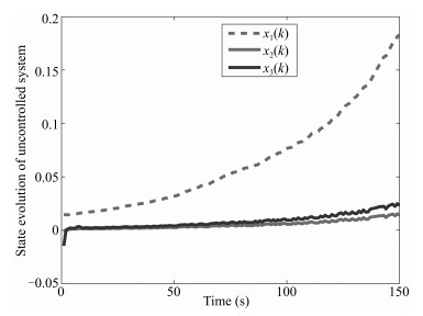 图 2 State evolution $x(k)$ of uncontrolled systems.Fig. 2 State evolution $x(k)$ of uncontrolled systems.
 图 3 State evolution $x(k)$ of controlled systems.Fig. 3 State evolution $x(k)$ of controlled systems.
In order to illustrate the disturbance-attenuation performance, we take the external disturbance
$ \begin{align*} v(k)= \begin{cases} 0.3,&20\leq k\leq 30 \\ -0.2,&50\leq k\leq 60 \\ 0,&\hbox{else}. \end{cases} \end{align*} $
Fig. 4 presents the controller-state evolution $x_c(k)$, Fig. 5 plots the state evolution of the controlled output $z(k)$, and Fig. 6 shows the output feedback controller. From Figs. 3$-$6, one can see that the convergence rate is rapid and effective. By the above simulation results, we can draw the conclusion that our theoretical analysis to the robust $H_\infty$ fuzzy-control problem is right completely.
Remark 2: The above simulation is performed on the basis of the software MATLAB 7.0 and the cone-complementarity linearization algorithm may takes several minutes because of choosing initial feasible set.
6. Conclusion
In this paper, we establish general networked systems model with multiple time-varying random communication delays and multiple missing measurements as weil as the random missing control and discuss its robust $H_\infty$ fuzzy-output feedback-control problem. The proposed system model includes parameter uncertainties, multiple stochastic time-varying delays, multiple missing measurements, and stochastic control input missing. The control strategy adopts the parallel distributed compensation. We obtain the sufficient conditions on the robustly exponential stability of the closed-loop T-S fuzzy-control system by using the CCL algorithm and the explicit expression of the desired controller parameters. An illustrative simulation example further shows that the fuzzy-control method to the proposed new control model is feasible and the new control model can be used for future applications. Whether to construct piecewise Lyapunov functions [8] to solve the proposed control model or not is an interesting topic and in active thought.
-

图 10 $\alpha$和$\beta$对收敛时间的影响
Fig. 10 Influence of $\alpha$ and $\beta$ on convergence time

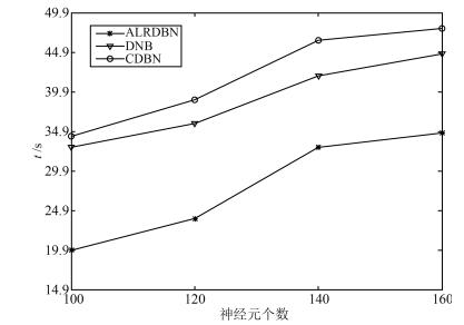
图 14 隐含层神经元数对收敛时间的影响
Fig. 14 Effect of the number of hidden neurons on convergence time
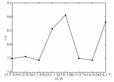
图 15 $\alpha$和$\beta$对收敛时间的影响
Fig. 15 Influence of $\alpha$ and $\beta$ on convergence time
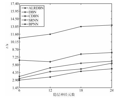
图 19 隐含层神经元数对收敛时间的影响
Fig. 19 Effect of the number of hidden neurons on convergence time

图 20 $\alpha$和$\beta$对收敛时间的影响
Fig. 20 Influence of $\alpha$ and $\beta$ on convergence time
表 1 MNIST手写数字实验结果对比
Table 1 Result comparison of MNIST experiment
方法 隐含层数 每层节点数 正确识别率 运算时间(s) ALRDBN 2 100 93.1 % 20.0 CDBN 2 100 93.0 % 34.3 DBN[21] 2 100 92.6 % 32.9  下载: 导出CSV
-
[1] Bengio Y H, Delalleau O. On the expressive power of deep Architectures. In:Proceeding of the 22nd International Conference. Berlin Heidelberg, Germany:Springer-Verlag, 2011. 18-36 [2] Hinton G E, Salakhutdinov R R. Reducing the dimensionality of data with neural networks. Science, 2006, 313(5786):504-507 doi: 10.1126/science.1127647 [3] 郭潇逍, 李程, 梅俏竹.深度学习在游戏中的应用.自动化学报, 2016, 42(5):676-684 http://www.aas.net.cn/CN/abstract/abstract18857.shtmlGuo Xiao-Xiao, Li Cheng, Mei Qiao-Zhu. Deep learning applied to games. Acta Automatica Sinica, 2016, 42(5):676-684 http://www.aas.net.cn/CN/abstract/abstract18857.shtml [4] LeCun Y, Bengio Y, Hinton G. Deep learning. Nature, 2015, 521(7553):436-444 doi: 10.1038/nature14539 [5] 贺昱曜, 李宝奇.一种组合型的深度学习模型学习率策略.自动化学报, 2016, 42(6):953-958 http://www.aas.net.cn/CN/abstract/abstract18886.shtmlHe Yu-Yao, Li Bao-Qi. A combinatory form learning rate scheduling for deep learning model. Acta Automatica Sinica, 2016, 42(6):953-958 http://www.aas.net.cn/CN/abstract/abstract18886.shtml [6] 马帅, 沈韬, 王瑞琦, 赖华, 余正涛.基于深层信念网络的太赫兹光谱识别.光谱学与光谱分析, 2015, 35(12):3325-3329 http://cdmd.cnki.com.cn/Article/CDMD-10674-1015636153.htmMa Shuai, Shen Tao, Wang Rui-Qi, Lai Hua, Yu Zheng-Tao. Terahertz spectroscopic identification with deep belief network. Spectroscopy and Spectral Analysis, 2015, 35(12):3325-3329 http://cdmd.cnki.com.cn/Article/CDMD-10674-1015636153.htm [7] 耿志强, 张怡康.一种基于胶质细胞链的改进深度信念网络模型.自动化学报, 2016, 42(6):943-952 http://www.aas.net.cn/CN/abstract/abstract18885.shtmlGeng Zhi-Qiang, Zhang Yi-Kang. An improved deep belief network inspired by glia chains. Acta Automatica Sinica, 2016, 42(6):943-952 http://www.aas.net.cn/CN/abstract/abstract18885.shtml [8] Abdel-Zaher A M, Eldeib A M. Breast cancer classification using deep belief networks. Expert Systems with Applications, 2016, 46:139-144 doi: 10.1016/j.eswa.2015.10.015 [9] Rumelhart D E, Hinton G E, Williams R J. Learning representations by back-propagating errors. Nature, 1986, 323(6088):533-536 doi: 10.1038/323533a0 [10] Mohamed A R, Dahl G E, Hinton G. Acoustic modeling using deep belief networks. IEEE Transactions on Audio, Speech, and Language Processing, 2012, 20(1):14-22 doi: 10.1109/TASL.2011.2109382 [11] Bengio Y. Learning deep architectures for AI. Foundations and Trends in Machine Learning, 2009, 2(1):1-127 doi: 10.1561/2200000006 [12] Lopes N, Ribeiro B. Improving convergence of restricted Boltzmann machines via a learning adaptive step size. Progress in Pattern Recognition, Image Analysis, Computer Vision, and Applications, Lecture Notes in Computer Science. Berlin Heidelberg:Springer, 2012. 511-518 [13] Raina R, Madhavan A, Ng A Y. Large-scale deep unsupervised learning using graphics processors. In:Proceedings of the 26th Annual International Conference on Machine Learning. New York, NY, USA:ACM, 2009. 873-880 [14] Ly D L, Paprotski V, Danny Y. Neural Networks on GPUs:Restricted Boltzmann Machines, Technical Report, University of Toronto, Canada, 2009. [15] Lopes N, Ribeiro B. Towards adaptive learning with improved convergence of deep belief networks on graphics processing units. Pattern Recognition, 2014, 47(1):114-127 doi: 10.1016/j.patcog.2013.06.029 [16] Le Roux N, Bengio Y. Representational power of restricted boltzmann machines and deep belief networks. Neural Computation, 2008, 20(6):1631-1649 doi: 10.1162/neco.2008.04-07-510 [17] Hinton G E. Training products of experts by minimizing contrastive divergence. Neural Computation, 2002, 14(8):1771-1800 doi: 10.1162/089976602760128018 [18] Yu X H, Chen G A, Cheng S X. Dynamic learning rate optimization of the backpropagation algorithm. IEEE Transactions on Neural Networks, 1995, 6(3):669-677 doi: 10.1109/72.377972 [19] Magoulas G D, Vrahatis M N, Androulakis G S. Improving the convergence of the backpropagation algorithm using learning rate adaptation methods. Neural Computation, 1999, 11(7):1769-1796 doi: 10.1162/089976699300016223 [20] Lee H, Ekanadham C, Ng A. Sparse deep belief net model for visual area V2. In:Proceedings of the 2008 Advances in Neural Information Processing Systems. Cambridge, MA:MIT Press, 2008. 873-880 [21] Ji N N, Zhang J S, Zhang C X. A sparse-response deep belief network based on rate distortion theory. Pattern Recognition, 2014, 47(9):3179-3191 doi: 10.1016/j.patcog.2014.03.025 [22] 乔俊飞, 潘广源, 韩红桂.一种连续型深度信念网的设计与应用.自动化学报, 2015, 41(12):2138-2146 http://www.aas.net.cn/CN/abstract/abstract18786.shtmlQiao Jun-Fei, Pan Guang-Yuan, Han Hong-Gui. Design and application of continuous deep belief network. Acta Automatica Sinica, 2015, 41(12):2138-2146 http://www.aas.net.cn/CN/abstract/abstract18786.shtml [23] Chang L C, Chen P A, Chang F J. Reinforced two-step-ahead weight adjustment technique for online training of recurrent neural networks. IEEE Transactions on Neural Networks and Learning Systems, 2012, 23(8):1269-1278 doi: 10.1109/TNNLS.2012.2200695 [24] Chen Q L, Chai W, Qiao J F. A stable online self-constructing recurrent neural network. Advances in Neural Networks-ISNN 2011. Berlin Heidelberg:Springer, 2011, 6677:122-131 期刊类型引用(4)
1. 练红海,肖伸平,罗毅平,周笔锋. 基于T-S模糊模型的采样系统鲁棒耗散控制. 自动化学报. 2022(11): 2852-2862 .  本站查看
本站查看2. 顾晓清,倪彤光,张聪,戴臣超,王洪元. 结构辨识和参数优化协同学习的概率TSK模糊系统. 自动化学报. 2021(02): 349-362 . 本站查看3. 李军,黄卫剑,万文军,刘哲. 一种新型反馈控制器的研究与应用. 控制理论与应用. 2020(02): 411-422 . 百度学术4. 唐晓铭,邓梨,虞继敏,屈洪春. 基于区间二型T-S模糊模型的网络控制系统的输出反馈预测控制. 自动化学报. 2019(03): 604-616 . 本站查看其他类型引用(1)
-

 下载:
下载:


计量
- 文章访问数: 2882
- HTML全文浏览量: 381
- PDF下载量: 1288
- 被引次数: 5
