

-
摘要: 互联系统的容错控制是近年来控制领域的研究热点,具有重要的理论价值和实际意义.本文阐述了互联系统容错控制的基本结构和主要思想,总结了带有机械互联、网络互联和模型虚拟互联的三类互联系统的容错控制最新研究成果,并对该研究方向进行了展望.Abstract: Fault tolerant control (FTC) of interconnected systems is a remarkable aspect of the control field in recent years, which has both important academic and engineering values. This paper introduces the basic structure and main idea of the FTC design for interconnected systems, and makes a comprehensive review of the recent theoretical results on the FTC of systems with mechanical interconnections, network interconnections, and model virtual interconnections. Some perspectives are also provided.
-
DC-DC变换器是指能完成直流电路电压转换的电力电子装置, 目前主要应用于直流电压转换、开关电源、直流电机驱动等场合.从功能上来区分, DC-DC变换器可以分为Buck变换器 (降压)、Boost变换器 (升压)、Boost-Buck变换器 (升--降压) 和Buck-Boost变换器 (降--升压) [1].随着现代工业技术的发展, 对直流变换器的要求越来越高, 既要求系统轻便、稳定、可靠, 又要求系统有较高的动态性能.由于DC-DC变换器是一类典型的开关非线性系统, 传统的线性控制设计方法很难保证系统较高的性能.因此, 结合DC-DC变换器模型特点, 研究先进的非线性控制方法已成为电力电子变换器系统研究的一个重要内容.本文主要针对Buck变换器, 提出一种新的非线性控制方法, 以实现电压的快速调节.
目前, 已有不少文献展开对Buck变换器的非线性控制方法研究.文献[2 $-$ 5]分别利用反步法、自适应控制、滑模控制、模糊控制对DC-DC变换器系统设计非线性控制算法, 以提高闭环系统的性能.文献[6]提出通过构造Lyapunov函数来分析和设计一类电力电子变换器的非线性控制系统.文献[7]利用非线性函数设计非线性PI控制器, 比传统线性PI有更好的调节效果和控制性能.文献[8]利用非线性采样输出反馈理论, 设计了一类针对Buck变换器的非线性控制算法, 以提高系统的鲁棒性.文献[9]利用扩展状态观测器, 设计了一类针对Buck变换器的非线性滑模控制算法, 提高了系统抗负载突变的能力.
值得指出的是, 前述所提及的非线性控制算法基本上都要求闭环系统满足局部利普希兹条件, 从而只能保证闭环系统的渐近稳定性[10].从收敛性角度来说, 在实际应用中, 更希望电压能在有限时间内收敛到参考电压.近年来, 有限时间控制算法作为一种新发展的非线性控制算法, 它可以保证闭环系统状态在有限时间内收敛到平衡点.目前, 这种控制方法在理论界[11-16]和应用界[17-23]已得到了广泛的关注.此外, 对于Buck变换器而言, 由于其外部负载常随时间而变化, 如何提高闭环系统抗负载变化能力也是控制算法设计关注的焦点问题之一.当系统存在干扰时, 有限时间控制算法还具有较强的抗负载变化能力, 具体见文献[24]中的理论分析以及文献[17]中的实验验证.文献[25]基于终端滑模控制技术, 对Buck变换器系统设计了有限时间控制器, 但该文献并没有考虑输入饱和受限和负载未知情况.
本文主要针对Buck变换器系统模型特点, 基于有限时间控制理论, 设计了一类有界的非线性自适应控制算法, 以实现电压的快速调节, 并同时满足系统对占空比函数有界约束的要求.首先, 基于时间尺度变换, 引入一个可调的参数, 得到变换后的系统; 然后, 通过构造合适的Lyapunov函数, 设计一类饱和的有限时间控制器; 最后, 利用齐次性理论, 得出系统是有限时间稳定的结论, 即输出电压在有限时间内收敛到参考电压.对负载未知情况, 基于有限时间观测器理论, 设计了自适应控制方法, 以实现对未知负载的估计.本文最后给出仿真实验结果, 并与PI控制算法进行了性能对比.仿真结果表明, 所提出的控制算法使得系统既具有较快的响应速度又有较强的抗负载变化能力.
1. 模型介绍及预备知识
1.1 Buck型DC-DC变换器系统模型
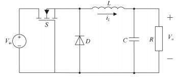
Buck型DC-DC变换器工作原理如图 1所示, 其中 $V_{\rm in}$ 是输入电压, $V_o$ 是输出电压, $S$ 是MOS型开关, $D$ 是二极管, $L$ 、 $C$ 、 $R$ 分别是电感、电容和负载电阻, $i_L$ 是电感电流.在开关频率足够快的情况下, DC-DC变换器可以近似为一般的状态空间模型, 其状态方程为[4]:
$ \begin{align}\label{zhtfc} &\dot i_L=\frac{1}{L} (\mu V_{\rm in}-V_o)\notag\\ &\dot V_o=\frac{1}{C} \left(i_L-\frac{V_o}{R}\right) \end{align} $
(1) 其中, $\mu$ 是控制输入, 即为MOS型开关管 $S$ 的占空比, $\mu \in [0, 1]$ .
假设 $V_{\rm ref}$ 为期望参考输出电压.令 $x_1=V_{\rm ref}-V_o$ 为输出电压误差, 则可以得到误差动态方程为
$ \begin{align}\label{wcdtfc} &\dot x_1=x_2=-\frac{{\rm d}V_o}{{\rm d}t}\notag\\ &\dot x_2=-\frac{1}{LC}x_1-\frac{1}{RC}x_2-\frac{V_{\rm in}}{LC}\mu +\frac{V_{\rm ref}}{LC}\notag\\ &y=x_1 \end{align} $
(2) 1.2 时间尺度坐标变换
为便于控制器设计, 对方程 (2) 进行时间尺度的坐标变换.令 $t=Ms$ , 其中 $M$ 为待设计的一个正常数.定义坐标变换:
$ \begin{align}\label{zbbh} &z_1(s)=x_1(Ms)=x_1(t)\notag \\ &z_2(s)=Mx_2(Ms)=Mx_2(t)\notag \\ &u(s)=M^2\mu(Ms)=M^2\mu(t) \end{align} $
(3) 那么根据式 (2) 可得:
$ \begin{align}\label{bianxing} &\frac{{\rm d}z_1(s)}{{\rm d}s}=\frac{{\rm d}x_1(Ms)}{{\rm d}s}=Mx_2(Ms)=z_2(s)\notag \\ &\quad\frac{{\rm d}z_2(s)}{{\rm d}s}=M\frac{{\rm d}x_2(Ms)}{{\rm d}s}=\notag\\ &\quad -\frac{1}{LC}M^2z_1(s)-\frac{1}{RC}Mz_2(s)-\notag\\ &\quad \frac{V_{\rm in}}{LC}u(s)+\frac{V_{\rm ref}}{LC}M^2 \end{align} $
(4) 为了便于设计控制器, 令
$ \begin{align}\label{canshutihuan} &b_1=\frac{1}{LC}M^2\notag \\ &b_2=\frac{1}{RC}M\notag \\ &f(s)=-\frac{V_{\rm in}}{LC}u(s)+\frac{V_{\rm ref}}{LC}M^2 \end{align} $
(5) 则方程 (2) 可简化为
$ \begin{align}\label{huajianmoxing} &\frac{{\rm d}z_1(s)}{{\rm d}s}=z_2(s)\notag \\ &\frac{{\rm d}z_2(s)}{{\rm d}s}=-b_1z_1(s)-b_2z_2(s)+f(s) \end{align} $
(6) 其中, $b_1>0, b_2>0$ , $f(s)$ 是控制器.
1.3 相关定义和引理
定义1.为了书写方便, 记
$ \begin{align}\label{sig} sig^\alpha(x)={\rm sgn}(x) |x|^\alpha \end{align} $
(7) 其中, $\alpha\geq0$ , $x\in \boldsymbol{R}$ , ${\rm sgn}(\cdot)$ 为符号函数.
定义2.定义一类新的饱和函数
$ \begin{align} sat_{\alpha}(x)=\left\{ {\begin{array}{*{20}c} { {\rm sgn}(x), |x|>1} \\ sig^\alpha(x), |x|\leq1 \end{array}} \right. \end{align} $
(8) 其中, $0\leq\alpha\leq1$ , $x\in \boldsymbol{R}$ .
定义3[4].令 $f(x)=(f_1(x), \cdots, f_n(x))^{\rm T}:{{\mathbf{R}}^{n}}\rightarrow {\bf R}^n$ 为一向量函数.若对任意的 $\varepsilon>0$ , 存在 $(r_1, \cdots, r_n)$ , 其中 $r_i>0, i=1, \cdots, n, $ 使得 $f(x)$ 满足:
$ f_i(\varepsilon^{r_1}x_1, \cdots, \varepsilon^{r_n}x_n)=\varepsilon^{k+r_i}f_i(x), \quad i=1, \cdots, n $
其中, $k>-{\rm min}\{r_i, i=1, \cdots, n\}$ , 则称 $f(s)$ 关于 $(r_1, \cdots, r_n)$ 具有齐次度 $k$ , 其中 $(r_1, \cdots, r_n)$ 称为扩张.
定义4[24].考虑系统
$ \begin{align} \dot x=f(x), x \in U \subseteq {{\mathbf{R}}^{n}}, f(0)=0 \end{align} $
(9) 其中, $f:U\rightarrow \boldsymbol{R}^n$ 为开区域 $U$ 上对 $x$ 连续的函数, 且开区域 $U$ 包含原点.系统的解 $x=0$ 为有限时间稳定当且仅当系统是稳定的且为有限时间收敛的.所谓有限时间收敛指的是:对 $\forall x_0\in U_0\subset {\bf R}^n$ , 存在一个连续函数 $T(x):U_0\setminus\{0\}\rightarrow(0, +\infty)$ , 使得系统 (9) 的解 $x(t, x_0)$ 满足:当 $t\in [0, T(x_0))$ 时, 有 $x(t, x_0)\in U_0\setminus{\{0\}}$ 和 $\lim\nolimits_{x\to T(x_0)}x(t, x_0)=0$ ; 当 $t>T(x_0)$ 时, 有 $x(t, x_0)=0$ .若 $U=U_0={\bf R}^n$ , 则系统是全局有限时间稳定的.
引理1[26].对于如下系统
$ \begin{align} \dot x=f(x)+\hat f(x), \quad x\in {{\mathbf{R}}^{n}} \end{align} $
(10) 其中, $f(x)$ 是连续的齐次向量空间, 且针对扩张 $(r_1, \cdots, r_n)$ 具有齐次度 $k < 0$ , 函数 $\hat f(x)$ 满足 $\hat f(0)=0$ .如果 $x=0$ 是系统 $\dot x=f(x)$ 的渐近稳定平衡点, 且对 $\forall x\neq0$ ,
$ \begin{align} \frac{\hat f_i(\varepsilon^{r_1}x_1, \cdots, \varepsilon^{r_n}x_{n})}{\varepsilon^{r_i+k}}=0, \quad i=1, 2, \cdots, n \end{align} $
(11) 那么 $x=0$ 是系统 (10) 的一个局部有限时间平衡点.如果系统 (10) 既是全局渐近稳定的, 又是局部有限时间稳定的, 那么它是全局有限时间稳定的.
2. 饱和有限时间控制器设计
在本节中, 主要针对坐标变换后的系统 (6) 进行饱和有限时间控制器设计.简便起见, 本节中省略的变量求导都是针对变量 $s$ .
定理1.对于系统 (6), 如果控制器设计成
$ \begin{align} f=-k_1sat_{\alpha_1}(z_1)-k_2sat_{\alpha_2}(z_2) \end{align} $
(12) 其中, $k_1 > 0, k_2 > 0, 0 < \alpha_1 < 1, \alpha_2=2\alpha_1/(1+\alpha_1)$ , 那么系统 (6) 的状态可以在有限时间被镇定到原点, 即在有限时间内, $(z_1(s), z_2(s))=0$ .
证明.证明可分为两个步骤.
步骤1. {证明全局渐近稳定性}
取Lyapunov函数:
$ \begin{align} V=k_1\int_0^{z_1}sat_{\alpha_1}(\rho){\rm d}\rho+\frac{1}{2}b_1z_1^2+\frac{1}{2}z_2^2 \end{align} $
(13) 由于 $\frac{{\rm d}\int_0^{z_1}sat_{\alpha_1}(\rho){\rm d}\rho}{{\rm d}s}=sat_{\alpha_1}(z_1)\dot z_1$ , 那么
$ \begin{align} &\dot V|_{(6)}=k_1sat_{\alpha_1}(z_1)z_2+b_1z_1z_2-b_1z_1z_2-b_2z_2^2+z_2f=\notag\\ &\quad k_1sat_{\alpha_1}(z_1)z_2-b_2z_2^2+z_2f \end{align} $
(14) 在所设计的控制器 (12) 作用下, 可得:
$ \begin{align} &\dot V|_{(6)-(12)}=k_1sat_{\alpha_1}(z_1)z_2-b_2z_2^2-\notag\\ &\quad k_1z_2sat_{\alpha_1}(z_1)-k_2z_2sat_{\alpha_2}(z_2)=\notag\\ &\quad -b_2z_2^2-k_2z_2sat_{\alpha_2}(z_2) \end{align} $
(15) 当 $|z_2|>1$ 时, $z_2sat_{\alpha_2}(z_2)=|z_2|$ , 当 $|z_2|\leq1$ 时, $z_2sat_{\alpha_2}(z_2)=|z_2|^{\alpha_2+1}$ , 故 $\dot V\leq0$ .
记集合 $\Psi=\{(z_1, z_2)|\dot V\equiv0\}$ .由式 (15) 可知 $\dot V\equiv0$ 意味着 $z_2\equiv0$ .亦即 $\dot z_2\equiv0$ .进一步根据式 (6) 和式 (12), 可以得到 $-b_1z_1-k_1sat_{\alpha_1}(z_1)\equiv0$ .注意到 $b_1, k_1$ 为正的增益, 从而 $z_1\equiv0$ .因此, 根据LaSalle不变集原理[27], 可以得出, 当 $s\to0$ 时, $(z_1(s), z_2(s))\to0$ , 即系统 (6) 在控制器 (12) 作用下是渐近稳定的.
步骤2.证明局部有限时间稳定
将闭环系统 (6) 和 (12) 重新写成如下形式:
$ \begin{align} &\dot z_1=z_2\notag\\ &\dot z_2=-k_1sat_{\alpha_1}(z_1)-k_2sat_{\alpha_2}(z_2)+g(z_1, z_2) \end{align} $
(16) 其中, $g(z_1, z_2)=-b_1z_1-b_2z_2$ .
由步骤1证明可知, 系统 (16) 是全局渐近稳定的, 那么系统的状态 $(z_1, z_2)$ 在有限时间内进入区域 $|z_1|\leq1, |z_2|\leq1$ .由饱和函数定义2, 此时系统 (16) 退化成为如下形式:
$ \begin{align} &\dot z_1=z_2\notag\\ &\dot z_2=-k_1sig^{\alpha_1}(z_1)-k_2sig^{\alpha_2}(z_2)+g(z_1, z_2) \end{align} $
(17) 对于系统 (17) 的标称系统:
$ \begin{align} \dot z_1&=z_2\notag\\ \dot z_2&=-k_1sig^{\alpha_1}(z_1)-k_2sig^{\alpha_2}(z_2) \end{align} $
(18) 构造Lyapunov函数如下:
$ \begin{align} W=k_1\int_0^{z_1}sig^{\alpha_1}(\rho) {\rm d}\rho+\frac {1}{2}z_2^2 \end{align} $
(19) 沿着系统 (18), 对式 (19) 进行求导, 得:
$ \begin{align} \dot W|_{(18)}=-k_2z_2sig^{\alpha_2}(z_2)=-k_2|z_2|^{\alpha_2+1} \end{align} $
(20) 故 $\dot W\leq0$ .
通过和步骤1类似的证明, 可以证明对于系统 (18), 当 $s\to\infty$ 时, 有 $(z_1(s), z_2(s))\to0$ , 亦即系统 (18) 是渐近稳定的.
另外由于 $0 < \alpha_1 < 1, \alpha_2=2\alpha_1/(1+\alpha_1)$ , 根据齐次性定义 (即定义3), 可知系统 (18) 的齐次度为 $m=(\alpha_1-1)/2 < 0$ , 其中 $r_1=1, r_2=(\alpha_1+1)/2$ .
接下来证明对于 $\forall(z_1, z_2)\neq(0, 0)$ , 有:
$ \lim\limits_{\varepsilon\to0}\frac{g(\varepsilon^{r_1}z_1, \varepsilon^{r_2}z_2)}{\varepsilon^{r_2+m}}=0 $
根据函数 $g(\cdot)$ 的定义, 有:
$ \begin{align} &\lim\limits_{\varepsilon\to0}\frac{g(\varepsilon^{r_1}z_1, \varepsilon^{r_2}z_2)}{\varepsilon^{r_2+m}}= \lim\limits_{\varepsilon\to0}\frac{-b_1\varepsilon^{r_1}z_1-b_2\varepsilon^{r_2}z_2}{\varepsilon^{r_2+m}}=\notag\\ &\quad \lim\limits_{\varepsilon\to0}(-b_1\varepsilon^{r_1-r_2-m}z_1-b_2\varepsilon^{-m}z_2)\notag \end{align} $
因为 $r_1 > r_2, m < 0$ , 所以 $\lim\nolimits_{\varepsilon\to0}(-b_1\varepsilon^{r_1-r_2-m}z_1-b_2\varepsilon^{-m}z_2)=0$ , 即 $\lim\nolimits_{\varepsilon\to0}\frac{g(\varepsilon^{r_1}z_1, \varepsilon^{r_2}z_2)}{\varepsilon^{r_2+m}}=0$ .因此, 根据引理1可知, 系统 (17) 是全局有限时间稳定的, 亦即系统 (16) 是局部有限时间稳定的.综合步骤1和步骤2, 可以得出系统 (6) 在控制器 (12) 的作用下是全局有限时间稳定.
注1.很显然, 所设计的控制器 (12) 是有界的.根据饱和函数的定义2, 可知 $|f|\leq k_1+k_2$ .因此, 为了满足实际系统对控制器饱和约束的条件, 可以调节控制参数 $k_1, k_2$ 满足任何约束条件.
3. Buck变换器快速有限时间降压控制算法设计
定理2.对于Buck型变换器系统 (1), 如果占空比函数设计成
$ \begin{align} \mu(t)=\frac{V_{\rm ref}}{V_{\rm in}}+\frac{LC}{M^2V_{\rm in}}[k_1sat_{\alpha_1}(x_1(t))+k_2sat_{\alpha_2}(M\cdot x_2(t))] \end{align} $
(21) 其中, $k_1 > 0, k_2 > 0, 0 < \alpha_1 < 1, \alpha_2=2\alpha_1/(1+\alpha_1)$ , 那么系统的输出电压 $V_o$ 可以在有限时间内达到参考电压 $V_{\rm ref}$ .
证明.首先, 对于所设计的控制器 (21), 在时间尺度 $t=Ms$ 变换下有:
$ \begin{align} &\mu(Ms)=\frac{V_{\rm ref}}{V_{\rm in}}+\frac{LC}{M^2V_{\rm in}}[k_1sat_{\alpha_1}(x_1(Ms))+\notag\\ &\quad k_2sat_{\alpha_2}(M\cdot x_2(Ms))] \end{align} $
(22) 在式 (22) 两边同时乘以 $M^2$ , 有:
$ \begin{align} &M^2\cdot\mu(Ms)=\frac{V_{\rm ref}}{V_{\rm in}}M^2+\frac{LC}{V_{\rm in}}[k_1sat_{\alpha_1}(x_1(Ms))+\notag\\ &\quad k_2sat_{\alpha_2}(M\cdot x_2(Ms))] \end{align} $
(23) 基于坐标变换 (3), 可得:
$ \begin{align} u(s)=\frac{V_{\rm ref}}{V_{\rm in}}M^2+\frac{LC}{V_{\rm in}}[k_1sat_{\alpha_1}(z_1(s))+k_2sat_{\alpha_2}(z_2(s))] \end{align} $
(24) 进一步, 根据式 (5) 可得:
$ \begin{align} &f(s)=-\frac{V_{\rm in}}{LC}u(s)+\frac{V_{\rm ref}}{LC}M^2=\notag\\ &\quad -k_1sat_{\alpha_1}(z_1(s))-k_2sat_{\alpha_2}(z_2(s)) \end{align} $
(25) 因此, 基于定理1, 可证明系统 (1) 在控制器 (21) 作用下是全局有限时间稳定的, 即输出电压 $V_o$ 能在有限时间内稳定到参考电压 $V_{\rm ref}$ .
注2.对于所设计的占空比函数 (21), 其大小满足:
$ \begin{align} \frac{V_{\rm ref}}{V_{\rm in}}-\frac{LC}{M^2V_{\rm in}}(k_1+k_2)\leq\mu\leq\frac{V_{\rm ref}}{V_{\rm in}}+\frac{LC}{M^2V_{\rm in}}(k_1+k_2) \end{align} $
(26) 由于 $0 < V_{\rm ref}/V_{\rm in} < 1$ , 因此很方便调节参数 $M, k_1, k_2$ 保证 $0 < \mu < 1$ .
4. Buck变换器快速自适应有限时间降压控制算法设计
本节中, 将考虑负载电阻突变情况下的有限时间降压控制算法设计问题.根据式 (1) 和 (2) 可知, 为了获得状态 $x_2$ , 需要精确知道负载 $R$ .然而实际中负载往往是随时间而变化的.接下来将主要基于有限时间观测器技术对未知负载在有限时间内估计其精确值.
令 $\hat R$ 为未知负载 $R$ 的估计值.为了便于设计, 令 $\theta=-1/R$ 为未知的参数, 令 $\hat\theta$ 为其估计值.
定理3.对于Buck变换器的未知负载电阻, 如果估计器设计为
$ \begin{align} &\dot{\hat{V}}_o=\frac{1}{C}(i_L+\hat\theta V_o)+l_1V_osig^{\beta_1}(V_o-\hat{V}_o)\notag\\ &\dot{\hat{\theta}}=l_2V_osig^{\beta_2}(V_o-\hat{V}_o) \end{align} $
(27) 那么估计值 $\hat\theta$ (或 $\hat R=-1/\hat\theta$ ) 在有限时间内收敛到真实值 $\theta$ (或 $R$ ), 其中 $l_1, l_2$ 为合适的正增益, $0.5 < \beta_1 < 1, \beta_2=2\beta_1-1$ .
证明.定义估计器误差
$ \begin{align} e_1=V_o-\hat{V}_o, e_2=\theta-\hat\theta \end{align} $
(28) 注意到 $\theta$ 是一个常数, 那么根据式 (27) 和 (28) 可得:
$ \begin{align} &\dot{\hat{e}}_1=\frac{V_o}{C}e_2-l_1V_osig^{\beta_1}(e_1)\notag\\ &\dot{\hat{e}}_2=-l_2V_osig^{\beta_2}(e_1) \end{align} $
(29) 基于文献[28]中的定理3.1, 可知存在合适的增益使得该系统是有限时间收敛的, 即估计值 $\hat\theta$ 在有限时间内收敛到真实值 $\theta$ , 亦即负载估计值 $\hat R=-1/\hat \theta$ 在有限时间内收敛到真实负载 $R$ .
基于定理3, 针对Buck变换器负载未知情况, 根据式 (1)、(2) 和式 (21), 可以设计自适应有限时间控制算法的形式如下:
$ \begin{align} &\mu (t)=\frac{V_{\rm ref}}{V_{\rm in}}+\frac{LC}{M^2V_{\rm in}} [k_1sat_{\alpha_1}(x_1(t))+k_2sat_{\alpha_2}(M\hat x_2)]=\notag\\ &\quad \frac{V_{\rm ref}}{V_{\rm in}}+\frac{LC}{M^2V_{\rm in}}[k_1sat_{\alpha_1}(V_{\rm ref}-V_o)+\notag\\ &\quad k_2sat_{\alpha_2}\left[\frac {M}{C}\left(\frac{V_o}{\hat R}-i_L\right)\right] \end{align} $
(30) 图 2给出了自适应有限时间电压调节控制算法框图.
 图 2 自适应有限时间电压调节控制算法实现框图Fig. 2 The block diagram of adaptive finite-time voltage control algorithm
5. 仿真实验
本实验采用针对电力电子及电机拖动开发的专用仿真软件PSIM (Power simulation) 软件进行仿真, 控制策略图见图 2, 其中三角波的频率选择100 kHz.
5.1 系统仿真参数
在仿真中Buck变换器的参数选取为:输入电压 $V_{\rm in}=12$ V, 电感值 $L=5$ mH, 电容值 $C=1 000 \mu$ F, 负载电阻值 $R=30 \Omega$ , 输出参考电压 $V_{\rm ref}=8$ V.为了进行对比, 采用自适应有限时间控制 (Automatic frequency control, AFC) 与PI (Proportional integral control) 控制两种算法.
对于自适应有限时间控制算法式 (30) 和 (27), 参数值分别选为: $M=0.001$ , $k_1=0.225$ , $k_2=1, \alpha_1=1/5$ , $l_1=160$ , $l_2=6, \beta_1=0.55$ .
对于PI控制算法, 其比例和积分增益分别为 $K_P=0.1$ , $K_I=0.05$ .
分别考虑在启动过程、参考电压变化以及负载突变情况下系统动态响应性能.
5.2 参考电压变化情况下动态响应
负载保持30 $\Omega$ 不变, 参考电压在1 s时从8 V变化到5 V, 其他参数保持不变.系统动态响应波形见图 3.可以明显看出, 所提出的快速有限时间电压控制算法对参考电压变化的响应速度明显优于PI控制, 其中AFC控制的系统在开始启动时的调节时间是0.007 s, 1 s时参考电压变化时的调节时间是0.06 s; PI控制系统在开始启动时的调节时间是0.32 s, 1 s时参考电压变化时的调节时间是0.24 s.
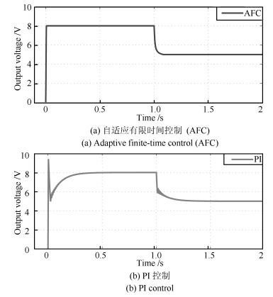 图 3 两种控制算法作用下输出电压响应曲线 (1 s时, 参考电压由8 V $\to$ 5 V)Fig. 3 The response curves for output voltage under two control algorithms (At 1 second, reference voltage is from 8 V $\to$ 5 V.)
5.3 负载突变情况下动态响应
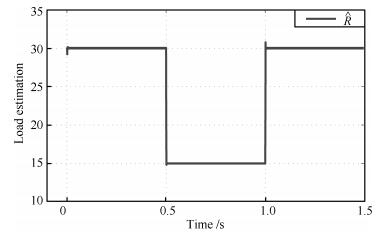
负载电阻变化如下:
$ \begin{align} {R}=\left\{ {\begin{array}{*{20}c} { {30}, 0\leq t\leq0.5 {\rm s}} \\ { {15}, 0.5 {\rm s} < t\leq1 {\rm s}} \\ { {30}, t > 1 {\rm s}} \\ \end{array}} \right. \end{align} $
(31) 其他参数保持不变.可以得到系统响应如图 4.负载电阻估计值响应曲线如图 5.
 图 4 两种控制算法作用下输出电压响应曲线 (0.5 s时, 负载电阻由30 $\Omega\to15 \Omega$ ; 1 s时, 负载电阻由15 $\Omega\to30 \Omega$ )Fig. 4 The response curves for output voltage under two control algorithms (At 0.5 second, load resistance is from 30 $\Omega\to15 \Omega$ ; at 1 second, load resistance is from 15 $\Omega\to30 \Omega$ .
AFC控制的系统在负载由30 $\Omega\to 15 \Omega$ 的调节时间为0.018 s, 电压波动范围为7.964 V $\sim$ 8 V, 在负载由15 $\Omega\to 30 \Omega$ 的调节时间为0.013 s, 电压波动范围为8 V $\sim$ 8.054 V。
PI控制的系统在负载由30 $\Omega\to 15 \Omega$ 的调节时间为0.034 s, 电压波动范围为7.631 V $\sim$ 8.365 V, 在负载由15 $\Omega\to 30 \Omega$ 的调节时间为0.048 s, 电压波动范围为7.628 V $\sim$ 8.368 V.
可见, 所提出的快速自适应有限时间降压控制方法对负载突变的响应更快, 电压波动更小.
上述结果表明, 相对于PI控制, 所提出的快速自适应有限时间降压控制算法具有较快的收敛性和较强的抗负载变化能力.
6. 结论
本文利用饱和有限时间控制和自适应控制理论设计出一类新的快速自适应降压控制算法, 使得即使负载未知情况下输出电压仍可以在有限时间内快速达到参考电压.通过构造Lyapunov函数从理论上严格证明了系统的全局有限时间稳定性.最后通过仿真对比, 验证了所提方法的有效性.
-

图 1 互联系统的容错控制结构
Fig. 1 The fault-tolerant control structure of the interconnected system
表 1 机械互联系统容错控制方法总结
Table 1 The summary of fault-tolerant control methods for systems with mechanical interconnections
互联系统特性 容错控制方法 实现方式 固定耦合 分布/分散式独立容错 调节故障子系统$i$的控制器$u_i$ 固定耦合 分布/分散式协同容错 综合调节故障子系统$i$和其他健康子系统 $j$的控制器$u_i$,$u_j$,$j\in M-\{i\}$ 耦合强度和
拓扑结构可变分布/分散式协同容错 综合调节故障子系统$i$和其他健康子系统 $j$的控制器$u_i$,$u_j$,$j\in M-\{i\}$
以及系统互联拓扑机构和耦合项组成可变 分布/分散式协同容错 重构子系统组成以及系统互联拓扑机构和耦合项  下载: 导出CSV
表 2 网络互联系统容错控制方法总结
Table 2 The summary of the fault-tolerant control methods for systems with network interconnections
互联系统特性 容错控制方法 实现方式 组成不变 分布/分散式独立容错 调节故障子系统$i$的控制器$u_i$以及子系统$i$获得信息的通信协议 组成不变 分布式协同容错 综合调节故障子系统$i$和其他健康子系统$j$的控制器${u_i},{u_j}$,$j\in M-\left\{ i \right\}$
以及这些子系统获得信息的通信协议组成可变 分布式协同容错 重构子系统组成以及系统网络拓扑机构和通信协议
下载: 导出CSV
-
[1] Antonelli G. Interconnected dynamic systems:an overview on distributed control. IEEE Control Systems, 2013, 33(1):76-88 doi: 10.1109/MCS.2012.2225929 [2] Patton R J, Kambhampati C, Casavola A, Zhang P, Ding S, Sauter D. A generic strategy for fault-tolerance in control systems distributed over a network. European Journal of Control, 2007, 13(2-3):280-296 doi: 10.3166/ejc.13.280-296 [3] Di Gennaro S. Output stabilization of flexible spacecraft with active vibration suppression. IEEE Transactions on Aerospace and Electronic Systems, 2003, 39(3):747-759 doi: 10.1109/TAES.2003.1238733 [4] Vournas C D, Papadias B C. Power system stabilization via parameter optimization-application to the Hellenic interconnected system. IEEE Transactions on Power Systems, 1987, 2(3):615-622 doi: 10.1109/TPWRS.1987.4335180 [5] Ren W, Beard R W, Atkins E M. Information consensus in multivehicle cooperative control. IEEE Control Systems, 2007, 27(2):71-82 doi: 10.1109/MCS.2007.338264 [6] Blanke M, Kinnaert M, Lunze J, Staroswiecki M. Diagnosis and Fault-Tolerant Control. Berlin:Springer, 2006. [7] 周东华, 叶银忠. 现代故障诊断与容错控制. 北京:清华大学出版社, 2000.Zhou Dong-Hua, Ye Yin-Zhong. Modern Fault Diagnosis and Fault-Tolerant Control. Beijing:Tsinghua University Press, 2000. [8] 胡昌华, 许化龙. 控制系统故障诊断与容错控制的分析和设计. 北京:国防工业出版社, 2000.Hu Chang-Hua, Xu Hua-Long. Design and Analysis of Fault-Tolerant Control and Fault Diagnosis for Control System. Beijing:National Defence Industry Press, 2000. [9] 姜斌, 冒泽慧, 杨浩, 张友民. 控制系统的故障诊断与故障调节. 北京:国防工业出版社, 2009.Jiang Bin, Mao Ze-Hui, Yang Hao, Zhang You-Min. Fault Diagnosis and Fault Regulation for Control Systems. Beijing:National Defence Industry Press, 2009. [10] Liu L, Wang Z S, Zhang H G. Adaptive fault-tolerant tracking control for MIMO discrete-time systems via reinforcement learning algorithm with less learning parameters. IEEE Transactions on Automation Science and Engineering, DOI:10.1109/TASE.2016.2517155, to be published [11] Wang Z S, Liu L, Zhang H G, Xiao G Y. Fault-tolerant controller design for a class of nonlinear MIMO discrete-time systems via online reinforcement learning algorithm. IEEE Transactions on Systems, Man, and Cybernetics:Systems, 2016, 46(5):611-622 doi: 10.1109/TSMC.2015.2478885 [12] Liu L, Wang Z S, Zhang H G. Adaptive NN fault-tolerant control for discrete-time systems in triangular forms with actuator fault. Neurocomputing, 2015, 152:209-221 doi: 10.1016/j.neucom.2014.10.076 [13] Khalil H K. Nonlinear Systems (3rd edition). Upper Saddle River, NJ:Prentice Hall, 2002. [14] Meskin N, Khorasani K. Actuator fault detection and isolation for a network of unmanned vehicles. IEEE Transactions on Automatic Control, 2009, 54(4):835-840 doi: 10.1109/TAC.2008.2009675 [15] Keliris C, Polycarpou M M, Parisini T. A distributed fault detection filtering approach for a class of interconnected continuous-time nonlinear systems. IEEE Transactions on Automatic Control, 2013, 58(8):2032-2047 doi: 10.1109/TAC.2013.2253231 [16] Zhang X D, Zhang Q. Distributed fault diagnosis in a class of interconnected nonlinear uncertain systems. International Journal of Control, 2012, 85(11):1644-1662 doi: 10.1080/00207179.2012.696146 [17] 郭志忠. 电网自愈控制方案. 电力系统自动化, 2005, 29(10):85-91 http://www.cnki.com.cn/Article/CJFDTOTAL-DLXT200510021.htmGuo Zhi-Zhong. Scheme of self-healing control frame of power grid. Automation of Electric Power Systems, 2005, 29(10):85-91 http://www.cnki.com.cn/Article/CJFDTOTAL-DLXT200510021.htm [18] 张颖伟, 刘建昌, 张嗣瀛. 一类复杂系统的容错控制. 控制与决策, 2005, 20(8):901-904, 908 http://www.cnki.com.cn/Article/CJFDTOTAL-KZYC200508012.htmZhang Ying-Wei, Liu Jian-Chang, Zhang Si-Ying. Reliable control for a class of interconnected systems. Control and Decision, 2005, 20(8):901-904, 908 http://www.cnki.com.cn/Article/CJFDTOTAL-KZYC200508012.htm [19] Panagi P, Polycarpou M M. Distributed fault accommodation for a class of interconnected nonlinear systems with partial communication. IEEE Transactions on Automatic Control, 2011, 56(12):2962-2967 doi: 10.1109/TAC.2011.2166313 [20] Panagi P, Polycarpou M M. A coordinated communication scheme for distributed fault tolerant control. IEEE Transactions on Industrial Informatics, 2013, 9(1):386-393 doi: 10.1109/TII.2012.2223220 [21] Jin X Z, Yang G H. Distributed adaptive robust tracking and model matching control with actuator faults and interconnection failures. International Journal of Control, Automation and Systems, 2009, 7(5):702-710 doi: 10.1007/s12555-009-0502-3 [22] Tong S C, Huo B Y, Li Y M. Observer-based adaptive decentralized fuzzy fault-tolerant control of nonlinear large-scale systems with actuator failures. IEEE Transactions on Fuzzy Systems, 2014, 22(1):1-15 doi: 10.1109/TFUZZ.2013.2241770 [23] Xiao B, Hu Q L, Zhang Y M. Fault-tolerant attitude control for flexible spacecraft without angular velocity magnitude measurement. Journal of Guidance, Control, and Dynamics, 2011, 34(5):1556-1561 doi: 10.2514/1.51148 [24] Panagi P, Polycarpou M M. Decentralized fault tolerant control of a class of interconnected nonlinear systems. IEEE Transactions on Automatic Control, 2011, 56(1):178-184 doi: 10.1109/TAC.2010.2089650 [25] 娄文涛, 佟绍成. 一类模糊T-S模型互联系统的自适应容错跟踪控制. 模糊系统与数学, 2014, 28(5):111-119 http://www.cnki.com.cn/Article/CJFDTOTAL-MUTE201405017.htmLou Wen-Tao, Tong Shao-Cheng. Adaptive fault-tolerant tracking control of fuzzy interconnected systems using Takagi-Sugeno fuzzy models. Fuzzy Systems and Mathematics, 2014, 28(5):111-119 http://www.cnki.com.cn/Article/CJFDTOTAL-MUTE201405017.htm [26] Hua C C, Li Y F, Wang H B, Guan X P. Decentralised fault-tolerant finite-time control for a class of interconnected non-linear systems. IET Control Theory and Applications, 2015, 9(16):2331-2339 doi: 10.1049/iet-cta.2014.1264 [27] Wang Z S, Li T S, Zhang H G. Fault tolerant synchronization for a class of complex interconnected neural networks with delay. International Journal of Adaptive Control and Signal Processing, 2014, 28(10):859-881 doi: 10.1002/acs.v28.10 [28] Yang H, Jiang B, Staroswiecki M, Zhang Y M. Fault recoverability and fault tolerant control for a class of interconnected nonlinear systems. Automatica, 2015, 54:49-55 doi: 10.1016/j.automatica.2015.01.037 [29] Liu T F, Hill D J, Jiang Z P. Lyapunov formulation of ISS cyclic-small-gain in continuous-time dynamical networks. Automatica, 2011, 47(9):2088-2093 doi: 10.1016/j.automatica.2011.06.018 [30] Godard, Kumar K D, Tan B. Fault-tolerant stabilization of a tethered satellite system using offset control. Journal of Spacecraft and Rockets, 2008, 45(5):1070-1084 doi: 10.2514/1.35029 [31] Bendtsen J, Trangbaek K, Stoustrup J. Plug-and-play control-modifying control systems online. IEEE Transactions on Control Systems Technology, 2013, 21(1):79-93 doi: 10.1109/TCST.2011.2174060 [32] Riverso S, Boem F, Ferrari-Trecate G, Parisini T. Fault diagnosis and control-reconfiguration in large-scale systems:a plug-and-play approach. In:Proceedings of the 53rd IEEE Conference on Decision and Control. Los Angeles, CA, USA:IEEE, 2014. 4977-4982 [33] Kambhampati C, Patton R J, Uppal F J. Reconfiguration in networked control systems:fault tolerant control and plug-and-play. In:Proceedings of the 6th IFAC Symposium on Fault Detection, Supervision, and Safety of Technical Processes. Beijing, China:IFAC, 2006. 126-131 [34] Yang H, Jiang B, Staroswiecki M. Fault tolerant control for plug-and-play interconnected nonlinear systems. Journal of the Franklin Institute, 2016, 353(10):2199-2217 doi: 10.1016/j.jfranklin.2016.04.001 [35] 张玮亚, 李永丽, 孙广宇, 靳伟, 李小叶. 微电网安全防御体系下电压分层分区控制. 电力系统自动化, 2015, 39(13):1-7, 15 http://www.cnki.com.cn/Article/CJFDTOTAL-DLXT201513001.htmZhang Wei-Ya, Li Yong-Li, Sun Guang-Yu, Jin Wei, Li Xiao-Ye. Hierarchical-partitioned voltage control under security safeguard system of microgrid. Automation of Electric Power Systems, 2015, 39(13):1-7, 15 http://www.cnki.com.cn/Article/CJFDTOTAL-DLXT201513001.htm [36] Guerraoui R, Schiper A. Software-based replication for fault tolerance. Computer, 1997, 30(4):68-74 doi: 10.1109/2.585156 [37] Guessoum Z, Briot J P, Marin O, Hamel A, Sens P. Dynamic and adaptive replication for large-scale reliable multi-agent systems. Software Engineering for Large-Scale Multi-Agent Systems. Heidelberg, Berlin:Springer, 2003. 182-198 [38] Guessoum Z, Faci N, Briot J P. Adaptive replication of large-scale multi-agent systems-towards a fault-tolerant multi-agent platform. Software Engineering for Large-Scale Multi-Agent Systems IV. Heidelberg, Berlin:Springer, 2006. 238-253 [39] Mellouli S. A reorganization strategy to build fault-tolerant multi-agent systems. Advances in Artificial Intelligence. Heidelberg, Berlin:Springer, 2007. 61-72 [40] Karimadini M, Lin H. Fault-tolerant cooperative tasking for multi-agent systems. International Journal of Control, 2011, 84(12):2092-2107 doi: 10.1080/00207179.2011.631149 [41] Bataineh S M, Allosl B Y. Fault-tolerant multistage interconnection network. Telecommunication Systems, 2001, 17(4):455-472 doi: 10.1023/A:1016779316848 [42] Bermond J C, Homobono N, Peyrat C. Large fault-tolerant interconnection networks. Graphs and Combinatorics, 1989, 5(1):107-123 doi: 10.1007/BF01788663 [43] Zhou B, Wang W, Ye H. Cooperative control for consensus of multi-agent systems with actuator faults. Computers and Electrical Engineering, 2014, 40(7):2154-2166 doi: 10.1016/j.compeleceng.2014.04.015 [44] Wang X, Yang G H. Cooperative adaptive fault-tolerant tracking control for a class of multi-agent systems with actuator failures and mismatched parameter uncertainties. IET Control Theory and Applications, 2015, 9(8):1274-1284 doi: 10.1049/iet-cta.2014.0700 [45] Ma H J, Yang G H. Adaptive fault tolerant control of cooperative heterogeneous systems with actuator faults and unreliable interconnections. IEEE Transactions on Automatic Control, 2016, 61(11):3240-3255 doi: 10.1109/TAC.2015.2507864 [46] Chen G, Song Y D. Robust fault-tolerant cooperative control of multi-agent systems:a constructive design method. Journal of the Franklin Institute, 2015, 352(10):4045-4066 doi: 10.1016/j.jfranklin.2015.05.031 [47] Shen Q K, Jiang B, Shi P, Zhao J. Cooperative adaptive fuzzy tracking control for networked unknown nonlinear multiagent systems with time-varying actuator faults. IEEE Transactions on Fuzzy Systems, 2014, 22(3):494-504 doi: 10.1109/TFUZZ.2013.2260757 [48] Zuo Z Q, Zhang J, Wang Y J. Adaptive fault-tolerant tracking control for linear and Lipschitz nonlinear multi-agent systems. IEEE Transactions on Industrial Electronics, 2015, 62(6):3923-3931 http://cn.bing.com/academic/profile?id=1d98b82030550a853913e31422100c4e&encoded=0&v=paper_preview&mkt=zh-cn [49] 王巍, 王丹, 彭周华. 不确定非线性多智能体系统的分布式容错协同控制. 控制与决策, 2015, 30(7):1303-1308 http://www.cnki.com.cn/Article/CJFDTOTAL-KZYC201507024.htmWang Wei, Wang Dan, Peng Zhou-Hua. Fault-tolerant control for synchronization of uncertain nonlinear multi-agent systems. Control and Decision, 2015, 30(7):1303-1308 http://www.cnki.com.cn/Article/CJFDTOTAL-KZYC201507024.htm [50] Lewis M A, Tan K H. High precision formation control of mobile robots using virtual structures. Autonomous Robots, 1997, 4(4):387-403 doi: 10.1023/A:1008814708459 [51] Xu Q, Yang H, Jiang B, Zhou D H, Zhang Y M. Fault tolerant formations control of UAVs subject to permanent and intermittent faults. Journal of Intelligent and Robotic Systems, 2014, 73(1-4):589-602 doi: 10.1007/s10846-013-9951-2 [52] Liu Z X, Yu X, Yuan C, Zhang Y M. Leader-follower formation control of unmanned aerial vehicles with fault tolerant and collision avoidance capabilities. In:Proceedings of the 2015 International Conference on Unmanned Aircraft Systems. Denver, CO, USA:IEEE, 2015. 1025-1030 [53] Semsar-Kazerooni E, Khorasani K. Team consensus for a network of unmanned vehicles in presence of actuator faults. IEEE Transactions on Control Systems Technology, 2010, 18(5):1155-1161 doi: 10.1109/TCST.2009.2032921 [54] Semsar-Kazerooni E, Khorasani K. Optimal consensus algorithms for cooperative team of agents subject to partial information. Automatica, 2008, 44(11):2766-2777 doi: 10.1016/j.automatica.2008.04.016 [55] 史建涛, 何潇, 周东华. 多机编队系统的协同容错控制. 上海交通大学学报, 2015, 49(6):819-824 http://www.cnki.com.cn/Article/CJFDTOTAL-SHJT201506014.htmShi Jian-Tao, He Xiao, Zhou Dong-Hua. Cooperative fault tolerant control for multi-vehicle systems. Journal of Shanghai Jiaotong University, 2015, 49(6):819-824 http://www.cnki.com.cn/Article/CJFDTOTAL-SHJT201506014.htm [56] Azizi S M, Khorasani K. Cooperative actuator fault accommodation in formation flight of unmanned vehicles using relative measurements. International Journal of Control, 2011, 84(5):876-894 doi: 10.1080/00207179.2011.582157 [57] Azizi S M, Khorasani K. A hierarchical architecture for cooperative actuator fault estimation and accommodation of formation flying satellites in deep space. IEEE Transactions on Aerospace and Electronic Systems, 2012, 48(2):1428-1450 doi: 10.1109/TAES.2012.6178071 [58] Tousi M M, Khorasani K. Optimal hybrid fault recovery in a team of unmanned aerial vehicles. Automatica, 2012, 48(2):410-418 doi: 10.1016/j.automatica.2011.07.006 [59] Saboori I, Khorasani K. Actuator fault accommodation strategy for a team of multi-agent systems subject to switching topology. Automatica, 2015, 62:200-207 doi: 10.1016/j.automatica.2015.09.025 [60] Yang H, Staroswiecki M, Jiang B, Liu J Y. Fault tolerant cooperative control for a class of nonlinear multi-agent systems. Systems and Control Letters, 2011, 60(4):271-277 doi: 10.1016/j.sysconle.2011.02.004 [61] Yu X, Liu Z X, Zhang Y M. Fault-tolerant formation control of multiple UAVs in the presence of actuator faults. International Journal of Robust and Nonlinear Control, 2015, 26(12):2668-2685 http://cn.bing.com/academic/profile?id=64b409ea807e9f89fc8eaa197e3c6ac8&encoded=0&v=paper_preview&mkt=zh-cn [62] Zhang Y M, Jiang J. Fault tolerant control system design with explicit consideration of performance degradation. IEEE Transactions on Aerospace and Electronic Systems, 2003, 39(3):838-848 doi: 10.1109/TAES.2003.1238740 [63] Wang Y J, Song Y D, Gao H, Lewis F L. Distributed fault-tolerant control of virtually and physically interconnected systems with application to high-speed trains under traction/braking failures. IEEE Transactions on Intelligent Transportation Systems, 2016, 17(2):535-545 doi: 10.1109/TITS.2015.2479922 [64] Giulietti F, Pollini L, Innocenti M. Autonomous formation flight. IEEE Control Systems, 2000, 20(6):34-44 doi: 10.1109/37.887447 [65] 石桂芬, 方华京. 基于相邻矩阵的多机器人编队容错控制. 华中科技大学学报(自然科学版), 2005, 33(3):39-42 http://www.cnki.com.cn/Article/CJFDTOTAL-HZLG200503015.htmShi Gui-Fen, Fang Hua-Jing. Fault tolerance of multi-robot formation based on adjacency matrix. Journal of Huazhong University of Science and Technology (Nature Science Edition), 2005, 33(3):39-42 http://www.cnki.com.cn/Article/CJFDTOTAL-HZLG200503015.htm [66] Zhang J H, Xu X M, Hong L, Yan Y Z. Consensus recovery of multi-agent systems subjected to failures. International Journal of Control, 2012, 85(3):280-286 doi: 10.1080/00207179.2011.646313 [67] Yang H, Jiang B, Cocquempot V, Chen M. Spacecraft formation stabilization and fault tolerance:a state-varying switched system approach. Systems and Control Letters, 2013, 62(9):715-722 doi: 10.1016/j.sysconle.2013.05.007 [68] Jiang B, Wang J L, Soh Y C. Robust fault diagnosis for a class of linear systems with uncertainty. Journal of Guidance, Control, and Dynamics, 1999, 22(5):736-740 doi: 10.2514/2.4448 [69] Jiang B, Staroswiecki M, Cocquempot V. Fault diagnosis based on adaptive observer for a class of non-linear systems with unknown parameters. International Journal of Control, 2004, 77(4):367-383 http://cn.bing.com/academic/profile?id=fc42a2c324b1e27c7d9233557988276d&encoded=0&v=paper_preview&mkt=zh-cn [70] Giridhar A, El-Farra N H. A unified framework for detection, isolation and compensation of actuator faults in uncertain particulate processes. Chemical Engineering Science, 2009, 64(12):2963-2977 doi: 10.1016/j.ces.2009.03.016 [71] Chamseddine A, Noura H. Sensor network design for complex systems. International Journal of Adaptive Control and Signal Processing, 2012, 26(6):496-515 doi: 10.1002/acs.1297 [72] Atassi A N, Khalil H K. A separation principle for the stabilization of a class of nonlinear systems. IEEE Transactions on Automatic Control, 1999, 44(9):1672-1687 doi: 10.1109/9.788534 [73] Du M, Mhaskar P. Isolation and handling of sensor faults in nonlinear systems. Automatica, 2014, 50(4):1066-1074 doi: 10.1016/j.automatica.2014.02.017 [74] Wang Y Q, Zhou D H, Gao F R. Robust fault-tolerant control of a class of non-minimum phase nonlinear processes. Journal of Process Control, 2007, 17(6):523-537 doi: 10.1016/j.jprocont.2006.12.002 [75] Yang H, Jiang B, Zhang H G. Stabilization of non-minimum phase switched nonlinear systems with application to multi-agent systems. Systems and Control Letters, 2012, 60(10):1023-1031 http://cn.bing.com/academic/profile?id=6cdb07571953c2e482569f840d7f35d8&encoded=0&v=paper_preview&mkt=zh-cn -

 下载:
下载:
计量
- 文章访问数: 2684
- HTML全文浏览量: 416
- PDF下载量: 1608
- 被引次数: 0
