2.845

2023影响因子

(CJCR)

  • 中文核心
  • EI
  • 中国科技核心
  • Scopus
  • CSCD
  • 英国科学文摘

留言板

尊敬的读者、作者、审稿人, 关于本刊的投稿、审稿、编辑和出版的任何问题, 您可以本页添加留言。我们将尽快给您答复。谢谢您的支持!

姓名
邮箱
手机号码
标题
留言内容
验证码

一类面向中风后吞咽功能障碍康复治疗的群体智慧涌现方法

宿翀 高月 李宏光 刘晓华

郭炳华, 戴宏跃, 李中华. 基于视觉注意的移动机器人环境3D建模. 自动化学报, 2017, 43(7): 1248-1256. doi: 10.16383/j.aas.2017.e150274
引用本文: 宿翀, 高月, 李宏光, 刘晓华. 一类面向中风后吞咽功能障碍康复治疗的群体智慧涌现方法. 自动化学报, 2017, 43(7): 1190-1201. doi: 10.16383/j.aas.2017.c160190
Guo Binghua, Dai Hongyue, Li Zhonghua. A Visual-attention-based 3D Mapping Method for Mobile Robots. ACTA AUTOMATICA SINICA, 2017, 43(7): 1248-1256. doi: 10.16383/j.aas.2017.e150274
Citation: SU Chong, GAO Yue, LI Hong-Guang, LIU Xiao-Hua. A Generating Approach to Group's Intelligence with Application to Dysphagia's Rehabilitation Treatment after Stroke. ACTA AUTOMATICA SINICA, 2017, 43(7): 1190-1201. doi: 10.16383/j.aas.2017.c160190

一类面向中风后吞咽功能障碍康复治疗的群体智慧涌现方法

doi: 10.16383/j.aas.2017.c160190
基金项目: 

国家自然科学基金 61603023

北京市优秀人才资助项目 2015000020124G041

中国科学院复杂系统管理与控制国家重点实验室开放课题 20150103

详细信息
    作者简介:

    宿翀 北京化工大学信息学院讲师.主要研究方向为人工智能, 情感计算和智能医疗.E-mail:suchong@mail.buct.edu.cn

    高月 北京化工大学信息学院硕士研究生.主要研究方向为智能决策.E-mail:18810255106@163.com

    李宏光:刘晓华 北京市积水潭医院物理康复科副主任医师.主要研究方向为康复医学诊疗.E-mail:bbjliuxhua@sina.com

    通讯作者:

    李宏光 北京化工大学信息学院教授.主要研究方向为化工过程的建模, 控制和优化.本文的通信作者.E-mail:lihg@mail.buct.edu.cn

A Generating Approach to Group's Intelligence with Application to Dysphagia's Rehabilitation Treatment after Stroke

Funds: 

Supported by National Natural Science Foundation of China 61603023

Beijing Outstanding Talent Training Project 2015000020124G041

Open Research Project from the State Key Laboratory of Management and Control for Complex Systems 20150103

More Information
    Author Bio:

     Lecturer at Beijing University of Chemical Technology. His research interest covers intelligent applications, afiect computing, and smart medicine

     Master student at Beijing University of Chemical Technology.Her main research interest is intelligent decision making

     Associate professor at Beijing Jishuitan Hospital. Her research interest covers diagnosis and treatment in rehabilitation medicine

    Corresponding author: LI Hong-Guang Professor at Beijing University of Chemical Technology. His research interest covers modeling, control and optimization of chemical process as well as computer based intelligent control for industrial plants. Corresponding author of this paper.E-mail:lihg@mail.buct.edu.cn
  • 摘要: 传统的中风后吞咽功能障碍康复治疗方案的制订通常以会诊方式,需要群体专家对所有可能的备选治疗方案进行讨论与决策,增加专家主观疲劳,且缺乏针对群体治疗智慧涌现方法的探讨,基层康复医师难以学习群体专家治疗智慧.基于多属性群决策理论,本文提出了群体智慧定义,给出了基于"专家讨论后的备选方案排序结果——子属性特征"的群体智慧涌现方法以及基于群体智慧的多属性决策方法,使计算机逐步学习群体专家经验并代替专家决策,减轻群体专家疲劳感,并具备针对未知备选方案进行自动决策的能力.针对一类数值实例,对传统多属性决策方法与所提决策方法进行了对比,并将所提方法应用于一类实际中风后吞咽功能障碍康复治疗中,验证了本文所提方法的正确性与可行性.
  • Environmental mapping has always been one of the most active areas in mobile robotics research for decades. Mobile robots use sensors to perceive the surrounding environment and build environment maps, which provide essential information for the navigation, localization, and path planning of mobile robots.

    Many scholars have been dedicated to the environment mapping research of mobile robots to promote their applications in various fields. The primary models of this field include metric models [1], topology models [2], and hybrid models [3], which are used in different environments. Metric models, which include occupancy grids and feature maps, are often applied to small environments, e.g., a room or a small building, and metrical methods are effective in building accurate geometrical models of small-scale environments. A topological map models the world as a collection of nodes, which can be paths or places. Thus, topological maps can describe a large-scale environment easily. However, topological representations lack details such as the structures associated with the nodes and the relationships described as links. Hybrid models combine the strengths of metrical and topological approaches and are suitable for modeling large-scale spaces. These proposed models are used to describe the environment with 2-D maps, which are widely adopted in mobile robots because of their relatively small computation requirements [4]-[6].

    Although 2-D maps have the advantages of simplicity and small computation, these maps provide limited information, particularly height information; thus, they are unsuitable for use in complex environments. For example, obstacles above the ground (mobile robots can pass through) are difficult to be described by using 2-D maps (e.g., four-legged tables in a room, hole-type passages, and external components of tunnels). Many researchers have expanded these 2-D representations to 3-D maps [7]-[10], which may be used to safely navigate a complex environment and perform other useful tasks (e.g., local localization).

    Point cloud models and voxel based grid models are the major existing 3-D models. For example, the 3-D laser mapping [11] and 3-D RGB-D camera mapping [12]. However, the huge amounts of data have to be processed for the point cloud model. It greatly reduces the efficiency of the system. Also, the point cloud data are easily influenced by noise and cause the accuracy of modeling to deteriorate. Grid maps are widely used in the environment modeling. However, the runtime and accuracy highly depend on the degree of discretization. Environment mapping for mobile robots brings great challenges, especially when robots work in an outdoor environment. For example, uncertainty of the environment, illumination variation, etc., which may deteriorate the accuracy of modeling. This paper uses the saliency based modeling to improve these performances in construction of environment 3-D maps.

    Visual attention is the ability of human vision system to rapidly select the most relevant information in the visual field [13]. In computer vision, the advancements obtained by simulating visual attention have accelerated the development of computer models. In some applications of mobile robots such as navigation, simultaneous localization and mapping (SLAM), and local planning, the robots need to model only nearby objects at every moment (we consider these objects as relevant) and not all the objects in the environment. Thus, visual attention models are suitable for mobile robots in modeling the environment. One of the most popular visual saliency models was proposed by Itti et al.[13], namely, the data-driven attention model, which computes the multi-scales feature contrasts of input images (such as intensity, color, and orientation features) by using a difference of Gaussian filter and linearly combines the features conspicuous maps to produce a master saliency map. After nearly 20 years of development, researchers have proposed many computational visual attention models [14], including Bayesian surprise models, task-driven models, etc. These models have been applied in many fields of robotics [15].

    Motivated by the advantages of visual attention models, we intend to apply these models to robot environment modeling. In this paper, we first present a visual saliency model that extracts the visual features from the scene and combines the features with the mean shift algorithm by using motion contrasts to detect the saliency of objects. We then adopt a stereo visual method and Bayesian estimation algorithm to construct and update the 3-D grid model of the environment. The evaluated system and the block diagram of the proposed method are shown in Figs. 1 and 2. The dash box in Fig. 2 is used to create the saliency model.

    图 1  The robot system used in our evaluations. (a) Mobile robot platform. (b) Binocular visual system and DM642 image processing card.
    Fig. 1  The robot system used in our evaluations. (a) Mobile robot platform. (b) Binocular visual system and DM642 image processing card.
    图 2  Schematic overview of the method. The dash box is used for saliency modeling construction, and a 3-D map is generated by using the probability of occupancy.
    Fig. 2  Schematic overview of the method. The dash box is used for saliency modeling construction, and a 3-D map is generated by using the probability of occupancy.

    The remainder of this paper is organized as follows. Section 2 provides an overview of related works. Section 3 describes the proposed visual saliency models. Section 4 explains the construction of the 3-D environment. Section 5 provides some experiments to verify the effectiveness of our proposed method. Finally, Section 5 concludes.

    Attention-driven visual saliency allows humans to focus on conspicuous objects. By utilizing this visual attention mechanism, mobile robots can be made to adapt to complex environments. Currently, visual saliency models are used in many fields of mobile robots, such as visual simultaneous localization and mapping (VSLAM), environment modeling, conspicuous object detection, and local localization [15].

    Extracting useful landmarks is one of the main tasks of VSLAM. Frintrop et al. [16] presented a method of selecting landmarks on the basis of attention-driven mechanisms that favor salient regions. The feature vectors of salient regions are considered landmarks, and their results have shown that their method facilitates the easy detection, matching, and tracing of landmarks compared with standard detectors such as Harris-Laplacians and scale-invariant feature transform (SIFT) key points. Newman et al. [17] used the entropy of the saliency field as landmarks and applied it to the loop-closing task. However, the features extracted with the saliency model are distinct and sparse and are unsuitable for environment mapping.

    Ouerhani et al. [18] adopted a multi-scale saliency-based model of visual attention to automatically acquire robust visual landmarks and constructed a topological map of the navigation environment. Einhorn et al. [19] applied attention-driven saliency models to 3-D environment modeling and mainly focus on the feature selection of image areas where the obstacle situation is unclear and a detailed scene reconstruction is necessary. Roberts et al. [20] presented an approach of tree mapping in unstructured outdoor environments for vision-based autonomous aerial robots. The visual attention models they used target the saliency of nearby trees and ignore innocuous objects that are far away from the robots. This approach is related to our work; however, the motion parallax was used to describe the saliency in these models and the camera rotation was to be estimated.

    Compared with 2-D maps, 3-D maps can provide detailed information and are suitable for mobile robot applications, such as local localization and navigation. Three-dimensional grid maps are one of the most used metric approaches because of their simplicity and suitability for all types of sensors. Souza et al. [7] used a grid occupancy probability method to construct the 3-D environment of mobile robots. They used stereo vision to interpret the depth of image pixels and deduce a sensorial uncertainty model related to the disparity to correct the 3-D maps; however, the cost of computation was expensive. By using the data acquired by laser range finders, Hähnel et al. [8] combined robot pose estimation with an algorithm to approximate environments by using flat surfaces to reconstruct the 3-D environment. Given the large data and to accelerate the computation, they used the split-and-merge technique to extract the lines out of the individual 2-D range scans; however, their method requires expensive laser sensors. Pirker et al. [9] presented a fast and accurate 3-D environment modeling method. They used depth image pyramids to accelerate the computation time and a weighted interpolation scheme between neighboring pyramids layers to boost the model accuracy. The algorithm is real time but is implemented on the GPU. Kim et al. [10] proposed a framework of building continuous occupancy maps. They used a coarse-to-fine clustering method and applied Gaussian processes to each local cluster to reduce the high-computational complexity. The experiment results with real 3-D data in large-scale environments show the feasibility of this method.

    Most saliency models compute primitive feature contrasts such as intensity, orientation, color, and others (e.g., edge gradient) to generate saliency, and these models are widely used for robots in landmark selection, and object tracking or location. However, these models are unsuitable for environment mapping. Our system uses motion contrasts to construct the saliency model, which is conducive for mapping close and conspicuous objects in the applications of robots such as navigation and VSLAM. In 3-D mapping, we approximate the saliency value as a priori information on the occupancy of the cell. This scheme avoids the need to train the grid occupancy maps created previously. Many objects exist in the visual scene of robots, and the selective mapping and priori information approximation of 3-D cells significantly improve the efficiency of system mapping and reduce interferences such as illumination changes.

    Cameras capture more detailed information in every moment than range finders, such as laser scanners. However, not all objects in the environment have an effect on mobile robots. For example, in the application of mobile robots such as navigation, only some nearby obstacles hinder the motion of mobile robots and objects that are far from the mobile robots have a minimal effect at times. If we only model the objects that have considerable effects on mobile robots in every moment, the entire system will be simplified. Visual saliency modeling (VSM) makes the robots focus on conspicuous objects. If the conspicuous objects are defined as nearby objects, environment modeling will be easily constructed.

    In the visual scene of mobile robots, only some objects in the environment affect the robots in a moment, e.g., objects that hinder the motion of mobile robots. Thus, the saliency model needs to highlight these conspicuous obstacles in the robot environment. Here, we use the distance between an obstacle and the mobile robot as the main parameters of saliency. The entire structure of the saliency model is shown in Fig. 2 in the dashed box.

    In the navigation of mobile robots, the scene captured by the visual system of the robots is always dynamic. Many previous works have focused on the detection of feature contrasts to trigger human vision nerves. This type of detection is usually referred to as the "stimuli-driven" mechanism. To detect nearby objects, we use a distance-potential function $\phi$ related to the distance r, i.e.,

    $ \begin{equation} \label{eq1} \phi =\frac{1}{2}k_p \left( {\frac{1}{r}-\frac{1}{r_0 }} \right)^2. \end{equation} $

    (1)

    Equation (1) shows that a smaller distance $r$ leads to a larger distance-potential $\phi$ . We define the distance-potential gradient of obstacles $s$ as follows:

    $ \begin{equation} \label{eq2} s=\frac{d\phi }{dt}=-k_p \left( {\frac{1}{r}-\frac{1}{r_0 }} \right)\frac{1}{r^2}\frac{dr}{dt}. \end{equation} $

    (2)

    Assume that the center coordinate of the mobile robot is $p(x, y, z)$ and that $p_i (x_i, y_i, z_i )$ is the point on the static obstacle. We can then obtain the following:

    $ r=\sqrt {(x_i-x)^2+(y_i-y)^2+(z_i-z)^2} . $

    By substituting $r$ in (2) and not considering the motion of the robot along the $z$ -axis (moves in a flat terrain), we obtain the following:

    $ \begin{equation} \label{eq3} s=-k_p \left( {\frac{1}{r}-\frac{1}{r_0 }} \right)\frac{1}{r^3}\left[{\left( {x_i-x} \right)v_x +\left( {y_i-y} \right)v_y } \right]. \end{equation} $

    (3)

    We model the motion contrast with (2) and consider the influence of the position of $p_i (x_i, y_i )$ . Thereafter, the saliency of $p_i$ can be defined as follows:

    $ \begin{equation} \label{eq4} {\rm sal} (p_i )=k_p k_d \left( {\frac{1}{r}-\frac{1}{r_0 }} \right)\frac{1}{r^3}\left[{\left( {x-x_i } \right)v_x +\left( {y-y_i } \right)v_y } \right] \end{equation} $

    (4)

    where $k_p$ is a normalization term and $r_0$ is the critical distance related to the speed of the mobile robot. $r_0$ can be obtained by experiments, and we determined that $r_0 =0.85$ in our experiments. $v_x$ and $v_y$ are the horizontal and vertical speeds of the mobile robot, respectively. The saliency of $p_i$ exhibits a higher value when the mobile robot moves closer to the obstacles with faster speed.

    $k_d $ in (4) is defined as the directional deviation of $p_i$ relative to the mobile robot (Fig. 3). We take as follows:

    图 3  The relation of $\Delta \varphi$ , $p$ ( $x$ , $y$ , $z$ ), and $p_i$ ( $x_i$ , $y_i$ , $z_i$ ), where $p$ ( $x$ , $y$ , $z$ ) is the center of the robot and $p_i$ ( $x_i$ , $y_i$ , $z_i$ ) is the feature point on the objects.
    Fig. 3  The relation of $\Delta \varphi$ , $p$ ( $x$ , $y$ , $z$ ), and $p_i$ ( $x_i$ , $y_i$ , $z_i$ ), where $p$ ( $x$ , $y$ , $z$ ) is the center of the robot and $p_i$ ( $x_i$ , $y_i$ , $z_i$ ) is the feature point on the objects.

    $ \begin{equation} \label{eq5} \Delta \varphi _i =\tan ^{-1}\left( {\frac{v_y }{v_x }} \right)-\tan ^{-1}\left( {\frac{y_i -y}{x_i -x}} \right). \end{equation} $

    (5)

    Equation (5) shows that point $p_i$ is located in front of the mobile robot when $\Delta \varphi =0$ . We normalize (5) as $k_d$ between $(-\pi, \pi )$ , then

    $ \begin{equation} \label{eq6} k_d =\left\{ {{\begin{array}{*{20}c} {1-\dfrac{\Delta \varphi _i }{\pi }}, \hfill \\ 1, \hfill \\ {1+\dfrac{\Delta \varphi _i }{\pi }}, \hfill \\ \end{array} }} \right.{\begin{array}{*{20}c} \hfill \\ \hfill \\ \hfill \\ \end{array} }{\begin{array}{*{20}c} \hfill \\ \hfill \\ \hfill \\ \end{array} }{\begin{array}{*{20}c} {\Delta \varphi >0} \hfill \\ {\Delta \varphi =0} \hfill \\ {\Delta \varphi <0} \hfill \\ \end{array} }. \end{equation} $

    (6)

    The motion saliency of points on obstacles can be calculated by using (4), and the result shows higher saliency when the mobile robot moves closer to the front obstacles.

    In (4) and (6), the position of points on objects can be acquired from the point cloud data obtained by using the stereo system. To reduce computational complexity, we use visual features such as SURF [21] or SIFT [22] to calculate the saliency of points. These features are widely used in the fields of image registration, matching, and object recognition because of their exceptional invariance performance in translation, rotation, scaling, lighting, and noise. The $v=(v_x, v_y )$ of the mobile robot can be obtained by using the output of the encoders coupled to the motors.

    Our target is to acquire the saliency of an object. Here, we use the conspicuous features to segment the objects. We first adopt the mean shift algorithm [23] to segment the objects and then use the conspicuous features to merge the segmented regions to generate the conspicuous objects. The mean shift algorithm is a robust feature-space analysis approach that can be applied to deal with discontinuity, preserving smoothing, and image segmentation problems. The algorithm uses an adaptive gradient ascent method to decompose an image into homogeneous tiles, and the mean shift procedure is not computationally expensive. The conspicuous objects acquired with the method will be applied to environment modeling.

    We use volumetric models [24] (3-D occupancy grid modeling) to construct the environment of mobile robots. The volumetric models adopt the occupancy of each independent cell to describe the position distribution of obstacles in the environment. These models have been extensively used in robotics because of their simplicity and suitability for various types of sensors. To reduce the uncertainty of mapping introduced by sensor noise, we use the probability of occupancy to model the environment of mobile robots.

    We suppose that the robotic environment workspace W is discreted into equally sized voxels $v_{i}$ with edge $\delta $ , and any edge of any voxel is assumed to be aligned with one of the axes of a global coordinate's frame [24]. We define the occupancy state of obstacle voxel $v_{i}$ as an independent random variable, and $p (v_{i})$ denotes the occupancy probability of the voxel occupied by an obstacle. The entire environment of mobile robots can be described as a probabilistic 3-D map, and the mobile robot uses the sensors to perceive the environment and acquires the data to update the map in the process of moving. Here, we apply Bayes' theorem [25] to update the probabilistic map. If we use $m$ to denote the measurement state, we obtain the following:

    $ \begin{equation} \label{eq7} p (v_i^t \vert m_i^t )=\frac{1}{\alpha }p(m_i^t \vert v_i^t )p(v_i^t \vert m_i^{t-1} ) \end{equation} $

    (7)

    where $t$ is the current time and $t-$ 1 is the last time. $\alpha $ is a normalization term and is related to the sensor model and is related to the priori information of voxel occupancy probability.

    Our mobile robot is equipped with a binocular stereo visual system, and the 3-D positions of points in the map coordinate frame can be calculated by using the robot pose and point disparity [26]. The error of position increases with distance because of the uncertainty of sensors. Reference [27] indicated that the error was proportional to the square of the distance:

    $ \begin{equation} \label{eq8} \Delta z=\frac{z^2}{Bf}\Delta d \end{equation} $

    (8)

    where $z$ is the depth of the feature points, and $\Delta z$ , $\Delta d$ are the depth error and disparity error respectively. $B$ is the stereo baseline, and $f$ is the focal length. In general, $\Delta d\approx 0.5$ . Assuming that the measurement error can be modeled by a Gaussian distribution, can be written as follows:

    $ \begin{equation} \label{eq9} p (m_i^t \vert v_i^t )=\frac{k_m }{\Delta r\sqrt {2\pi } }\exp \left[{-\frac{1}{2}\left( {\frac{r_i-\bar {r}}{\Delta r}} \right)^2} \right] \end{equation} $

    (9)

    where $\bar {r}=(\sum_{i=1}^N {r_i })/N$ , , $N$ is the number of features, $r$ denotes the measured distance of features, and $k_{m}$ is the normalization factor.

    A priori information about the occupancy of the cell can be obtained by training the grid occupancy maps created previously [25]; however, this procedure requires a large computation. Our proposed saliency model highlights nearby conspicuous objects in the robot environment and not all the objects. If we approximate the priori information with the feature saliency, it will reduce the cost of the computation. In (7), $p (v_i^t \vert m_i^{t-1} )$ is related to the priori information. To reduce the cost of the computation, we approximate the priori information with the feature saliency. Feature saliency describes the conspicuousness of feature points on obstacles. These points become larger when the mobile robot moves closer to the front feature points; hence, the occupancy probability of voxels contained in these feature points is similarly large. To make this approximation, we take $p (v_i^t \vert m_i^{t-1} )$ as follows:

    $ \begin{equation} \label{eq10} p (v_i^t \vert m_i^{t-1} )=\left\{ {{\begin{array}{*{20}c} {\zeta _i }, \hfill \\ {0.5}, \hfill \\ \end{array} }} \right.{\begin{array}{*{20}c} \hfill \\ \hfill \\ \end{array} }{\begin{array}{*{20}c} {z\le 3} \hfill \\ {z>3} \hfill \\ \end{array} } \end{equation} $

    (10)

    where $\zeta _i={\rm sal} (p_i )$ .

    We define the occupancy probability of a grid as 0.5 in (10) because the uncertainty of the sensors quickly increases with distance when the depth measured is over 3 m, i.e., it is an unknown state. We also approximate the probability by using the saliency value of the feature points.

    Three-dimensional grid modeling uses a space occupancy grid to describe the environment. In this section, we only discuss the static environment. We define obstacles as the static objects aboveground, such as the indoor wall, table, outdoor tree, and pillar.

    Our mobile robot is equipped with stereo vision. However, considering the installation's height restriction and that the mobile robot always detects objects from one side, occlusion will occur. Furthermore, identifying the grid occupancy state of entire object in maps will be difficult. We use the method of projection to calculate the occupancy range of the objects in the maps, and this method is shown in Fig. 4.

    图 4  Occupancy grid maps creation when objects produce visual occlusion. We use the projection method to calculate the objects occupancy width w.
    Fig. 4  Occupancy grid maps creation when objects produce visual occlusion. We use the projection method to calculate the objects occupancy width w.

    Fig. 4 is a side view of object projection. The shadow is an object that is divided into grid cells, and the others are the grid cells after projection. Suppose that the object occupancy width in a map is $w$ , the following can be expressed:

    $ \begin{equation} \label{eq11} w=\left\{ {{\begin{array}{*{20}c} {\dfrac{h_o D}{h_c -h_o }}, \hfill \\ \infty, \hfill \\ \end{array} }} \right.{\begin{array}{*{20}c} \hfill & {h_c >h_o } \hfill \\ \hfill & {h_c \le h_o } \hfill \\ \end{array} } \end{equation} $

    (11)

    where $h_c $ is the installation height of the cameras, $h_{o}$ is the object height, and $D$ is the distance from the object to camera. If $h_c \le h_o $ , the back of the objects cannot be detected. We then define $w=\infty $ . The length of objects can be obtained by using the mean shift segmentation algorithm [23], and its positions can be calculated by the stereo visual method.

    In mapping, the mobile robot must update the grid occupancy in time by using its visual system. The robot perceives the environment, obtains data, and calculates by using (7), (9), and (10). When the mobile robot finds the matching feature points (we only consider the features matching in the consecutive two images), the final updating can be conducted as follows:

    $ \begin{equation} \label{eq12} p (v_i^t \vert m_i^t )={\rm min}\left[{p (v_i^t \vert m_i^t ), p (v_i^{t-1} \vert m_i^{t-1} )} \right] \end{equation} $

    (12)

    where $p (v_i^t \vert m_i^t )$ and are the grid occupancies of the matching feature points in consecutive two images and min $[\cdot]$ is the obtained minimum. We used the projection method to calculate the grid occupancy of objects in the maps; hence, the occupancy range after projection may be larger than actual size of the objects. When a mobile robot moves from one position to another, the direction of the projection changes and we use (12) to correct these changes (Fig. 5). $A$ and $B$ are the two positions that the mobile robot passes in order, the arrows are the directions of the projection, and the shadows are the increasing area after projection. We use (12) to update the mobile robot moving from $A$ to $B$ , and the occupancy range of the objects decreases to be close to its actual size.

    图 5  Overhead view of occupancy grid updating. The updated results using (12) will be close to the size of objects when robot moves from $A$ to $B$ . The shadows are the occupancy fields of occlusion.
    Fig. 5  Overhead view of occupancy grid updating. The updated results using (12) will be close to the size of objects when robot moves from $A$ to $B$ . The shadows are the occupancy fields of occlusion.

    To decrease the mismatching features and remove the useless features, we add the following constraints to extract the matching features according to [8]:

    1) All the points in $Z=\pm 0.01$ are removed, where $Z$ is the height of feature points, thus implying that all feature points on the ground are discarded.

    2) All the matching points that do not meet the condition are removed as $\vert Z_1 -Z_2 \vert \le \delta _3 $ , where $Z_1 $ and $Z_2 $ are the heights of matching feature points, and we obtain $\delta _3 =0.05$ in our experiments.

    In the grid maps, we use the distance--potential gradient based on feature keypoints to calculate the saliency value of keypoints on nearby objects of the robot, and use these feature keypoints to describe the grid occupancy of the obstacles. However, when the number of these points is insufficient to describe the entire occupancy state of obstacles, these obstacles have to be segmented. We first use the mean shift algorithm [23] to segment the scenes scanned by cameras, and then combine these feature keypoints using similarity of features to segment these objects, and apply the stereo visual algorithm [26] to determine the positions of these objects.

    To verify the ability of the proposed method to construct the environment model, we perform a series of experiments containing VSM and indoor and outdoor environment mapping, and carry out some performance evaluation tests in different conditions. The whole 3-D map is constructed as the robot moving forward, and we use the method of keypoints matching in consecutive frames to avoid previously visited areas being re-mapped.

    In our experiments, the mobile robot we used is as shown in Fig. 1, and the ground is a plane. The mobile robot is equipped with a stereo camera pair, and the installation height of the cameras is $h_c =370$ mm. This value is used to compute the locations of the visual features of the environment. The computing hardware of the mobile robot includes a DM642 card with 600 MHz and an Intel Core i3 CPU with 2.40 GHz. The first installation is used for binocular stereo visual computation and feature extraction, whereas the other computational tasks are done by the Core i3 CPU, and these installations exchange data through network. $A_{\rm L}$ and are defined as the internal parameters of the left and right cameras, respectively, after calibration, and are given by the following:

    $ A_{\rm L} =\left[{{\begin{array}{*{20}ccccc} {1015.6} \hfill & ~~\!~~0 \hfill & {357.7} \hfill \\ ~~\!~~0 \hfill & {1073.5} \hfill & {264.3} \hfill \\ ~~\!~~0 \hfill & ~~\!~~0 \hfill & ~~\!~~1 \hfill \\ \end{array} }} \right] $

    $ A_{\rm R} =\left[{{\begin{array}{*{20}ccccc} {1037.0} \hfill & ~~\!~~0 \hfill & {339.0} \hfill \\ ~~\!~~0 \hfill & {1099.2} \hfill & {289.2} \hfill \\ ~~\!~~0 \hfill & ~~\!~~0 \hfill & ~~\!~~1 \hfill \\ \end{array} }} \right]. $

    The rotation matrix $R_{0}$ and translation matrix $T_{0}$ are given as follows:

    $ R_0 =\left[{{\begin{array}{*{20}cccccc} ~~\!~~1 \hfill & {-0.0059} \hfill & ~~{0.0060} \hfill \\ ~~{0.0062} \hfill & ~~{0.9987} \hfill & {-0.0503} \hfill \\ {-0.0057} \hfill & ~~{0.0503} \hfill & ~~{0.9987} \hfill \\ \end{array} }} \right] $

    $ T_0 =\left[{{\begin{array}{*{20}c} {-111.191} \hfill & {-1.395} \hfill & {6.279} \hfill \\ \end{array} }} \right]~~~~~ $

    where $A_{\rm L}$ , $A_{\rm R}$ , $R_{0}$ , and $T_{0}$ will be used in stereo visual computation. In our experiments, the speed of the mobile robot is limited to $v\le 0.5$ m/s.

    In the saliency modeling experiments, we use the visual features to construct the saliency maps. However, the number of features extracted from some objects may be not enough to show the saliency of these objects. Hence we first adopt the mean shift algorithm [23] to segment the objects, and then merge the segmented regions with these features to acquire the saliency of the objects. If the surface textures of the larger objects show a significant difference and are far apart from each other, the saliency may be different, as shown in Fig. 6.

    图 6  An example of a saliency map. (a) Conspicuous objects. Parts 1 and 3 are of the same object; however, because of the differences in texture and distance, the object was segmented into two parts. (b) Indoor corridor and conspicuous SURF features.
    Fig. 6  An example of a saliency map. (a) Conspicuous objects. Parts 1 and 3 are of the same object; however, because of the differences in texture and distance, the object was segmented into two parts. (b) Indoor corridor and conspicuous SURF features.

    Fig. 6(a) is a constructed visual saliency map with the conspicuous SURF features, and it is obtained by using (4) and (6) combined with the mean shift algorithm. In Fig. 6, the SURF features on ground have been removed. There are eight conspicuous regions in this figure, and first has the highest saliency and eighth has the least. In Region 1, the features are nearest to the mobile robot and have the smallest deviation relative to the moving direction of the robot. In Region 2, the features have smaller deviation, however, these are farther from the robot compared with Region 1. Hence the saliency in Region 2 is lower than Region 1. Regions 7 and 8 have a larger deviation and are far away from the robot, thus their saliency is the lowest. In right of Fig. 6(b) is the conspicuous SURF features map, and the saliencies of features are different.

    We first performed the 3-D grid modeling experiments in an indoor environment with a size of approximately 5.0 m $\times $ 6.5 m. The size of the grid is 0.1 m $\times $ 0.1 m $\times $ 0.1 m, and the grid modeling is mainly focused on conspicuous objects. The number of conspicuous visual features on the objects is inadequate, thus the objects contour formed by the voxels based on the features may not describe the actual occupancy situation of the objects in the environment, as shown in left portion of Fig. 7. The features are part of the map constructed by the SURF features (some closer features are combined together). In this figure, many grids show discontinuity because of the uneven distribution of features. To improve this situation, we first adopted the stereo visual method [26] to acquire the location of the objects with these features, and combined the mean shift segmentation algorithm and projection method to calculate the occupancy range of the objects in the map, as shown in Fig. 7(b) . The discontinuous grids are significantly reduced compared with Fig. 7(a) . Fig. 8 is an indoor corridor (see the left of Fig. 6(b)) 3-D grid map constructed by using our method, where the dashed line and arrow describe the path and moving direction of mobile robot, respectively.

    图 7  A part of 3-D occupancy grid map. (a) The map is created using SURF features, and many grids show discontinuity. (b) The map is created by combining the conspicuous SURF features with the mean shift algorithm, and the discontinuity is reduced significantly.
    Fig. 7  A part of 3-D occupancy grid map. (a) The map is created using SURF features, and many grids show discontinuity. (b) The map is created by combining the conspicuous SURF features with the mean shift algorithm, and the discontinuity is reduced significantly.
    图 8  Indoor corridor 3-D map with 1 dm $^3$ voxel size. The dash line and arrow are the trajectory and moving direction of mobile robot, respectively, and the small circles are the places used to evaluate the performance.
    Fig. 8  Indoor corridor 3-D map with 1 dm $^3$ voxel size. The dash line and arrow are the trajectory and moving direction of mobile robot, respectively, and the small circles are the places used to evaluate the performance.

    Fig. 9 is an outdoor 3-D grid map created with conspicuous SURF features, and the size of scene is approximately 30.5 m $\times $ 10 m. Some conspicuous objects are marked in map, such as trunks, pillars, cars, stone columns, and signboards, as shown in Fig. 9. Object 1 is a tree, and the positions of the tree leaves vary because of the effect of the wind, thus we limited the height of objects in the map as $h\!\!<$ 1.5 m, producing trunks with no leaves in the created map. The dashed line and arrow are the path and moving direction of mobile robot, respectively. The colors of the voxels indicate the heights in Figs. 8 and 9, such as gray: 0.1-0.2 m, white: 0.3-0.6 m, blue: 0.7-0.9 m, yellow: 1.0-1.2 m, red: 1.3-1.4 m.

    图 9  Outdoor 3-D map with 1 dm3 voxel size, where the dashed line and arrow are the trajectory and moving direction of mobile robot, respectively, and the little circles are the places used to evaluate the performance.
    Fig. 9  Outdoor 3-D map with 1 dm3 voxel size, where the dashed line and arrow are the trajectory and moving direction of mobile robot, respectively, and the little circles are the places used to evaluate the performance.

    In our method, we use the visual features to construct 3-D environment modeling, and the feature type is one of the most influential choices for accuracy and runtime performance. We use SIFT, SURF, and Harris-Laplace to evaluate our method in indoor and outdoor environments. Twenty places (see the circles in Figs. 8 and 9) are carefully selected to evaluate the performance. The plots in Fig. 10 show the processing time comparison per frame in indoor and outdoor environments, whereas Fig. 11 shows the mapping accuracy in these places. It is very difficult to evaluate all the mapping errors. We select 10 conspicuous feature points in specified locations (as shown in Figs. 8 and 9 and compute their mapping error. The comparison results clearly show that outdoor modeling requires more time and provides lower mapping accuracy than indoor modeling. More saliency features are extracted and some features easily become unstable because of the effect of light outdoors, particularly for the Harris-Laplace. In contrast, SIFT provides the highest accuracy (median is approximately 0.07 m), however, the processing time is also highest, and Harris-Laplace is the opposite. SURF offers a tradeoff choice for a robot with limited computational resources or applications that require real-time performance.

    图 10  Evaluation of runtime (a) indoor and (b) outdoor with respect to feature type. The plots have been generated from 20 places marked in the trajectory of the robot with small circles in Figs. 8 and 9.
    Fig. 10  Evaluation of runtime (a) indoor and (b) outdoor with respect to feature type. The plots have been generated from 20 places marked in the trajectory of the robot with small circles in Figs. 8 and 9.
    图 11  Evaluation of mapping accuracy (a) indoor and (b) outdoor with respect to feature type. The plots have been generated from 20 places marked on trajectory of robot with little circles in Figs. 8 and 9.
    Fig. 11  Evaluation of mapping accuracy (a) indoor and (b) outdoor with respect to feature type. The plots have been generated from 20 places marked on trajectory of robot with little circles in Figs. 8 and 9.

    Illumination changes may make the visual features become unstable, and the shadows of objects cast by light may change. These factors will cause false objects to occur in mapping, and reduce mapping accuracy. In our experiments, we evaluated the robust performance of the proposed method by the effects of light in an indoor environment. We control four lamps mounted on the ceiling to simulate illumination changes. In mapping, we use methods of VO (visual odometry) and SLAM to evaluate mapping accuracy, and the results are shown in Fig. 12. Results of experiments show that mapping accuracy deteriorates because of illumination, particularly the mapping error obtained using point clouds subsampling (PCS) (see the dash lines in Fig. 12). The solid lines are the results of our method, and it shows that the error reduces relatively little by the effects of light and shows good robust performance. This may be explained by the fact that the method of VSM gives priority to the closer objects when the robot is mapping the environment.

    图 12  Evaluation of mapping accuracy under (a) stable illumination and (b) varying illumination. The results are obtained with SURF and the mapping error increases under varying illumination, however, VSM slightly increases.
    Fig. 12  Evaluation of mapping accuracy under (a) stable illumination and (b) varying illumination. The results are obtained with SURF and the mapping error increases under varying illumination, however, VSM slightly increases.

    For the runtime, we compared our approach with some of the discussed approaches such as occupancy grid mapping (OGM) and occupancy mapping with pyramid (OMP) [9]. The experiments are performed in an indoor corridor shown in Fig. 6. The size of grid is 0.1 m 0.1 m $\times $ 0.1 m, and each moving distance of the mobile robot is approximately 8 m. The evaluation results are shown in Fig. 13. VSM significantly reduces mapping time, and OGM requires more time. For VSM, the mapping objects are the higher conspicuous objects, whereas other methods need to map all the objects scanned by the cameras. Hence this feature significantly improves the efficiency of mapping of VSM.

    图 13  Evaluation of runtime with VSM, OGM, and OMP. The results are obtained indoors, and the size of the grid is 0.1 m $\times$ 0.1 m $\times$ 0.1 m.
    Fig. 13  Evaluation of runtime with VSM, OGM, and OMP. The results are obtained indoors, and the size of the grid is 0.1 m $\times$ 0.1 m $\times$ 0.1 m.

    In this paper, we presented a method of 3-D grid modeling based on visual attention. VSM makes the front objects (that are closer to the mobile robots) exhibit larger conspicuousness. This can be beneficial for mobile robots to model the closer objects with higher priority, thus avoiding the modeling of all the objects at every moment, reducing computing time in updating the map of the environment. In the constructed method of VSM, we define the distance-potential gradient as the motion contrast, and combine the visual features with the mean shift segmentation algorithm to determine the saliency of the objects. To create the 3-D environment maps, we use stereo visual method to calculate the positions of conspicuous visual features and objects, and combine Bayes' theorem with the sensors modeling, grid priori modeling, and projection method to update the occupancy probability of the grids. Finally, a series of experiments that include saliency modeling, indoor and outdoor grid modeling, and performance tests are adopted to evaluate the presented method.


  • 本文责任编委 吕金虎
  • 图  1  中风后吞咽功能障碍治疗流程图

    Fig.  1  The treatment flow chart of dysphagia after stroke

    图  2  群体智慧涌现算法流程图

    Fig.  2  The flow chart of group intelligence algorithms

    图  3  子属性权重进化曲线

    Fig.  3  The evolutions of the sub-attribute's weight

    图  4  子属性可达区间下限的进化曲线

    Fig.  4  The evolutions of the sub-attribute's lower limit

    图  5  子属性可达区间上限的进化曲线

    Fig.  5  The evolutions of the sub-attribute's upper limit

    图  6  子属性权重进化曲线

    Fig.  6  The evolutions of the sub-attribute's weight

    图  7  子属性可达区间下限的进化曲线

    Fig.  7  The evolutions of the sub-attribute's lower limit

    图  8  子属性可达区间上限的进化曲线

    Fig.  8  The evolutions of the sub-attribute's upper limit

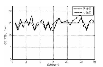
    图  9  基于所提决策方法与专家会诊的物理治疗时间对比图

    Fig.  9  The physical therapy time comparison chart based on the proposed decision method and expert consultation

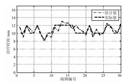
    图  10  基于所提决策方法与专家会诊的按摩时间对比图

    Fig.  10  The massage time comparison chart based on the proposed decision method and expert consultation

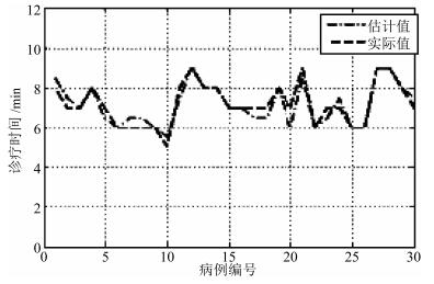
    图  11  基于所提决策方法与专家会诊的针灸时间对比图

    Fig.  11  The acupuncture time comparison chart based on the proposed decision method and expert consultation

    表  1  备选方案集

    Table  1  The alternatives

    u1u2u3
    x12.33.40.9
    x24.98.01.4
    x33.25.61.3
    x45.06.81.9
    x51.42.01.8
    下载: 导出CSV

    表  2  规范阵

    Table  2  The standard matrix

    u1u2u3
    S10.460.420.47
    S20.9810.74
    S30.640.70.68
    S410.851
    S50.280.250.95
    下载: 导出CSV

    表  3  备选方案集

    Table  3  The alternatives

    u1u2u3
    x1111217
    x214919
    x316518
    x412720
    下载: 导出CSV

    表  4  方案准确率对照表

    Table  4  The accuracy comparison of the treatment plan

    编号准确系数
    物理治疗按摩针灸平均
    11.000.850.940.93
    20.920.900.930.92
    30.901.001.000.97
    40.870.901.000.92
    50.901.000.930.94
    60.931.001.000.98
    70.80.950.920.89
    810.940.920.95
    90.90.9510.95
    1010.90.90.93
    下载: 导出CSV
  • [1] Hassan H E, Aboloyoun A I. The value of bedside tests in dysphagia evaluation. Egyptian Journal of Ear, Nose, Throat and Allied Sciences, 2014, 15 (3):197-203 doi: 10.1016/j.ejenta.2014.07.007
    [2] Navaneethan U, Eubanks S. Approach to patients with esophageal dysphagia. Surgical Clinics of North America, 2015, 95 (3):483-489 doi: 10.1016/j.suc.2015.02.004
    [3] Fields J, Go J T, Schulze K S. Pill properties that cause dysphagia and treatment failure. Current Therapeutic Research, 2015, 77:79-82 doi: 10.1016/j.curtheres.2015.08.002
    [4] Huang K L, Liu T Y, Huang Y C, Leong C P, Lin W C, Pong Y P. Functional outcome in acute stroke patients with oropharyngeal dysphagia after swallowing therapy. Journal of Stroke and Cerebrovascular Disease, 2014, 23 (10):2547-2553 doi: 10.1016/j.jstrokecerebrovasdis.2014.05.031
    [5] 庄福振, 罗平, 何清, 史忠植.迁移学习研究进展.软件学报, 2015, 26 (1):26-39 http://www.cnki.com.cn/Article/CJFDTOTAL-RJXB201501003.htm

    Zhuang Fu-Zhen, Luo Ping, He Qing, Shi Zhong-Zhi. Survey on transfer learning research. Journal of Software, 2015, 26 (1):26-39 http://www.cnki.com.cn/Article/CJFDTOTAL-RJXB201501003.htm
    [6] 范玉华, 秦世引.基于潜在语义分析的场景分类优化决策方法.计算机辅助设计与图形学学报, 2013, 25 (2):175-182 http://www.cnki.com.cn/Article/CJFDTOTAL-JSJF201302006.htm

    Fan Yu-Hua, Qin Shi-Yin. Optimizing decision for scene classification based on latent semantic analysis. Journal of Computer-aided Design and Computer Graphics, 2013, 25 (2):175-182 http://www.cnki.com.cn/Article/CJFDTOTAL-JSJF201302006.htm
    [7] 杨武夷, 曾智, 张树武, 李和平.基于人脸检测与SIFT的播音员镜头检测.软件学报, 2009, 20 (9):2417-2425 http://www.cnki.com.cn/Article/CJFDTOTAL-RJXB200909014.htm

    Yang Wu-Yi, Zeng Zhi, Zhang Shu-Wu, Li He-Ping. Anchor shot detection based on face detection and SIFT. Journal of Software, 2009, 20 (9):2417-2425 http://www.cnki.com.cn/Article/CJFDTOTAL-RJXB200909014.htm
    [8] 李琳辉, 郭景华, 张明恒, 连静.越野智能车转向及驱动协调控制.控制理论与应用, 2013, 30 (1):80-94 http://www.cnki.com.cn/Article/CJFDTOTAL-KZLY201301013.htm

    Li Lin-Hui, Guo Jing-Hua, Zhang Ming-Heng, Lian Jing. Coordinated control of steering and driving in off-road intelligent vehicle. Control Theory and Applications, 2013, 30 (1):80-94 http://www.cnki.com.cn/Article/CJFDTOTAL-KZLY201301013.htm
    [9] 李璐, 董秋雷, 赵瑞珍.含缺失成分的矩阵的广义低秩逼近及其在图像处理中的应用.计算机辅助设计与图形学学报, 2015, 27 (11):2065-2076 http://www.cnki.com.cn/Article/CJFDTOTAL-JSJF201511007.htm

    Li Lu, Dong Qiu-Lei, Zhao Rui-Zhen. Generalized low-rank approximations of matrices with missing components and its applications in image processing. Journal of Computer-Aided Design and Computer Graphics, 2015, 27 (11):2065-2076 http://www.cnki.com.cn/Article/CJFDTOTAL-JSJF201511007.htm
    [10] Yardimci A. Soft computing in medicine. Applied Soft Computing, 2009, 9 (3):1029-1043 doi: 10.1016/j.asoc.2009.02.003
    [11] Montani S. Exploring new roles for case-based reasoning in heterogeneous AI systems for medical decision support. Applied Intelligence, 2008, 28 (3):275-285 doi: 10.1007/s10489-007-0046-2
    [12] Yan H M, Jiang Y T, Zheng J, Peng C L, Li Q H. A multilayer perceptron-based medical decision support system for heart disease diagnosis. Expert Systems with Applications, 2006, 30 (2):272-281 doi: 10.1016/j.eswa.2005.07.022
    [13] Teodorescua H N L, Chelaru M, Kandel A, Tofan I, Irimia M. Fuzzy methods in tremor assessment, prediction, and rehabilitation. Artificial Intelligence in Medicine, 2001, 21 (1-3):107-130 doi: 10.1016/S0933-3657(00)00076-2
    [14] Shamsuddin S, Yussof H, Ismail L I, Mohamed S, Hanapiahc F A, Zaharid N I. Humanoid robot NAO interacting with autistic children of moderately impaired intelligence to augment communication skills. Procedia Engineering, 2014, 41:1533-1538
    [15] Zahedi Z M, Akbari R, Shokouhifar M, Safaei F, Jalali A. Swarm intelligence based fuzzy routing protocol for clustered wireless sensor networks. Expert Systems with Applications, 2016, 55:313-328 doi: 10.1016/j.eswa.2016.02.016
    [16] 何小贤, 朱云龙, 王玫.群体智能中的知识涌现与复杂适应性问题综述研究.信息与控制, 2005, 34 (5):560-566 http://www.cnki.com.cn/Article/CJFDTOTAL-XXYK200505010.htm

    He Xiao-Xian, Zhu Yun-Long, Wang Mei. Knowledge emergence and complex adaptability in swarm intelligence. Information and Control, 2005, 34 (5):560-566 http://www.cnki.com.cn/Article/CJFDTOTAL-XXYK200505010.htm
    [17] Sabir M M, Ali T. Optimal PID controller design through swarm intelligence algorithms for sun tracking system. Applied Mathematics and Computation, 2016, 274:690-699 doi: 10.1016/j.amc.2015.11.036
    [18] Nguyen D, Nguyen L T T, Vo B, Hong T P. A novel method for constrained class association rule mining. Information Sciences, 2015, 320:107-125 doi: 10.1016/j.ins.2015.05.006
    [19] Sahoo J, Das A K, Goswami A. An efficient approach for mining association rules from high utility itemsets. Expert Systems with Applications, 2015, 42 (13):5754-5778 doi: 10.1016/j.eswa.2015.02.051
    [20] 梁吉业, 冯晨娇, 宋鹏.大数据相关分析综述.计算机学报, 2016, 39(1):1-18 doi: 10.11897/SP.J.1016.2016.00001

    Liang Ji-Ye, Feng Chen-Jiao, Song Peng. A survey on correlation analysis of big data. Chinese Journal of Computers, 2016, 39 (1):1-18 doi: 10.11897/SP.J.1016.2016.00001
    [21] Ventura R, Pinto-Ferreir C. Responding efficiently to relevant stimuli using an affect-based agent architecture. Neurocomputing, 2009, 72 (13-15):2923-2930 doi: 10.1016/j.neucom.2008.09.019
    [22] Su C, Li H G. An affective learning agent with Petri-net-based implementation. Applied Intelligence, 2012, 37 (4):569-585 doi: 10.1007/s10489-012-0350-3
    [23] Su C, Li H G. A novel interactive preferential evolutionary method for controller tuning in chemical processes. Chinese Journal of Chemical Engineering, 2015, 23 (2):398-411 doi: 10.1016/j.cjche.2014.09.020
    [24] Su C, Li H G, Huang J W, Bao X Y. Generating methods for group affective preferences with engineering applications. Arabian Journal for Science and Engineering, 2015, 40 (6):1539-1551 doi: 10.1007/s13369-015-1617-x
    [25] 于超, 樊治平.指标期望为随机变量情形的多指标决策方法.控制与决策, 2015, 30 (8):1434-1440 http://www.cnki.com.cn/Article/CJFDTOTAL-KZYC201508015.htm

    Yu Chao, Fan Zhi-Ping. Multiple attribute decision making method with attribute aspirations in the form of random variable. Control and Decision, 2015, 30 (8):1434-1440 http://www.cnki.com.cn/Article/CJFDTOTAL-KZYC201508015.htm
    [26] 张小芝, 朱传喜, 朱丽.一种基于变权的动态多属性决策方法.控制与决策, 2014, 29 (3):494-498 http://www.cnki.com.cn/Article/CJFDTOTAL-KZYC201403018.htm

    Zhang Xiao-Zhi, Zhu Chuan-Xi, Zhu Li. A method of dynamic multi-attribute decision making based on variable weight. Control and Decision, 2014, 29 (3):494-498 http://www.cnki.com.cn/Article/CJFDTOTAL-KZYC201403018.htm
    [27] Xu Z S, Yager R R. Dynamic intuitionistic fuzzy multi-attribute decision making. International Journal of Approximate Reasoning, 2008, 48 (1):246-262 doi: 10.1016/j.ijar.2007.08.008
    [28] Ohmoto Y, Kataoka M, Nishida T. Extended methods to dynamically estimate emphasizing points for group decision-making and their evaluation. Procedia--Social and Behavioral Sciences, 2013, 97:147-155 doi: 10.1016/j.sbspro.2013.10.215
    [29] Meng F Y, Zhang Q. Induced continuous Choquet integral operators and their application to group decision making. Computers and Industrial Engineering, 2014, 68:42-53 doi: 10.1016/j.cie.2013.11.013
    [30] 姜艳萍, 樊治平.基于判断矩阵的决策理论与方法.北京:科学出版社, 2008. 74-78

    Jiang Yan-Ping, Fan Zhi-Ping. The Methods and the Theory of Decision Based on the Judge Matrix. Beijing:China Science Publishing and Media Ltd, 2008. 74-78
    [31] 徐泽水.不确定多属性决策方法及应用.北京:清华大学出版社, 2004.

    Xu Ze-Shui. Uncertain Multiple Attribute Decision Making:Method and Application. Beijing:Tsinghua University Press, 2004.
    [32] Xia M M, Xu Z S. Interval weight generation approaches for reciprocal relations. Applied Mathematical Modelling, 2014, 38 (3):828-838 doi: 10.1016/j.apm.2013.07.018
    [33] 倪延延, 张晋昕.向量自回归模型拟合与预测效果评价.中国卫生统计, 2014, 33 (1):53-56 http://www.cnki.com.cn/Article/CJFDTOTAL-ZGWT201401016.htm

    Ni Yan-Yan, Zhang Jin-Xin. Modeling and forecasting for multivariate time series using a vector autoregression model. Chinese Journal of Health Statistics, 2014, 33 (1):53-56 http://www.cnki.com.cn/Article/CJFDTOTAL-ZGWT201401016.htm
  • 加载中
  • 图(11) / 表(4)
    计量
    • 文章访问数:  1927
    • HTML全文浏览量:  136
    • PDF下载量:  693
    • 被引次数: 0
    出版历程
    • 收稿日期:  2016-03-03
    • 录用日期:  2016-11-03
    • 刊出日期:  2017-07-20

    目录

    /

    返回文章
    返回