

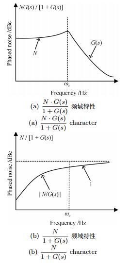
-
摘要: 频率合成源是射频发生和频谱分析中最重要的组成之一,评价合成源性能指标的是输出信号的相位噪声、杂散、频率分辨率和频率切换时间.本文通过分析传统锁相环原理,提出一种通用的超低相位噪声合成源设计方案(带宽100MHz以内).在锁相环基础上,通过引入直接数字合成(Direct digital synthesizer,DDS)混频鉴相技术,使得到的射频信号理论值达到0.1mHz的频率分辨率,同时将带内相位噪声指标优化17dB以上.新方案同时兼顾了杂散和频率切换时间指标,保障合成源的输出信号稳定可靠,使其在自动测试领域拥有广阔的应用前景.Abstract: Frequency synthesizer is one of the most important component of RF generator and spectrum analysis. The performance of its output signal is evaluated in terms of phase noise, scattering, frequency resolution and frequency hopping time. By analyzing the traditional theory of phase-locked loop, a ultralow-phase-noise scheme for the frequency synthesizer is put forward (bandwidth within 100MHz). In order to make the frequency resolution of the output signal reach to 0.1mHz in theory and optimize the in-band phase noise cver 17dB, direct digital synthesizer (DDS) and mixer phase detection technology based on phase-locked loop are introduced. Consideration is also given to both scattering and frequency hopping time to ensure the output signal is stable and reliable. The synthesizer has a good application in the field of automatic test.
-
Key words:
- Frequency synthesizer /
- phase-locked loop /
- high resolution /
- ultralow phase noise
1) 本文责任编委 辛景民 -

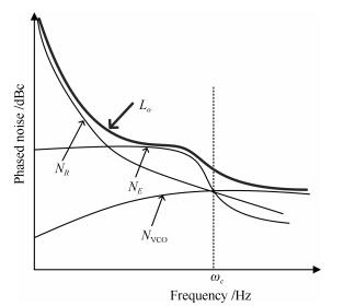
图 5 新方案各输入信号相噪表现
Fig. 5 Input Signals' phase noise spectrum performance in the new scheme

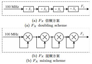
图 8 实际工程应用中$F_X$与$F_M$的产生方式
Fig. 8 The producing way of $F_X$ and $F_M$ in the practical engineering application
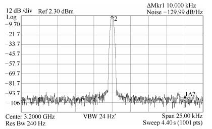
图 9 新方案$F_X=3 200$ MHz的相位噪声指标
Fig. 9 The phase noise curve of $F_X=3 200$ MHz in the new scheme
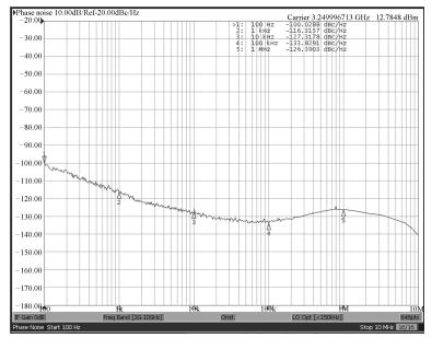
图 10 新方案$F_O$输出为3 250 MHz的相噪曲线
Fig. 10 The phase noise curve of the 3 250 MHz in the new scheme
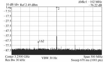
图 11 $F_O$ = 3 250 MHz时, 500 MHz以内杂散测试图
Fig. 11 The spurious test pattern at $F_O$ = 3 250 MHz within 500 MHz bandwidth
表 1 DDS频率切换时间
Table 1 DDS frequency hopping time
DDS切换频点(MHz) DDS切换时间($\mu$s) 107$\rightarrow$110 3.044 110$\rightarrow$113 3.022 113$\rightarrow$114 2.978 114$\rightarrow$121 3.044 121$\rightarrow$125 2.978 $\Delta$$T_{\rm DDS}$均值 3.013  下载: 导出CSV
表 2 环路切换时间
Table 2 Loop locked time
环路切换频点(MHz) 环路切换时间($\mu$s) 3 227$\rightarrow$3 232 13.67 3 232$\rightarrow$3 238 14.22 3 238$\rightarrow$3 240 15.00 3 240$\rightarrow$3 243 15.44 3 243$\rightarrow$3 248 14.00 $\Delta$$T_{\rm PLL}$均值 14.47
下载: 导出CSV
-
[1] 侯君锋. 多环路频率合成器的设计与实现[硕士学位论文], 电子科技大学, 中国, 2014 http://cdmd.cnki.com.cn/Article/CDMD-10614-1015701201.htmHou Jun-Feng. Design and Implementation of Multi-loop Frequency Synthesizer[Master dissertation], University of Electronic Science and Technology of China, China, 2014 http://cdmd.cnki.com.cn/Article/CDMD-10614-1015701201.htm [2] 陈丛宏. 低相噪X波段信号发生器的研究[硕士学位论文], 电子科技大学, 中国, 2014 http://cdmd.cnki.com.cn/Article/CDMD-10614-1015705743.htmChen Cong-Hong. The Research of Low Phase Niose X-band Signal Generator[Master dissertation], University of Electronic Science and Technology of China, China, 2014 http://cdmd.cnki.com.cn/Article/CDMD-10614-1015705743.htm [3] 程鹏.自动控制原理.北京:高等教育出版社, 2003. 35-57Cheng Peng. Principles of Automatic Control. Beijing:Higher Education Press, 2003. 35-57 [4] 储昭碧, 张崇巍, 冯小英.基于基波频率估计的多谐波分析.自动化学报, 2009, 35(5):532-539 http://www.aas.net.cn/CN/abstract/abstract15788.shtmlChu Zhao-Bi, Zhang Chong-Wei, Feng Xiao-Ying. Multi-harmonics analysis based on fundamental frequency estimate. Acta Automatica Sinica, 2009, 35(5):532-539 http://www.aas.net.cn/CN/abstract/abstract15788.shtml [5] 方涌. 8-10G低噪声频率综合器系统设计[硕士学位论文], 南京理工大学, 中国, 2011 http://cdmd.cnki.com.cn/Article/CDMD-10288-1011173193.htmFang Yong. Design of 8-10G Low Phase Noise Frequency Synthesizers[Master dissertation], Nanjing University of Science and Technology, China, 2011 http://cdmd.cnki.com.cn/Article/CDMD-10288-1011173193.htm [6] Mehrotra A. Noise analysis of phase-locked loops. IEEE Transactions on Circuits and Systems I:Fundamental Theory and Applications, 2002, 49(9):1309-1316 doi: 10.1109/TCSI.2002.802347 [7] Maffezzoni P, Levantino S. Analysis of VCO phase noise in charge-pump phase-locked loops. IEEE Transactions on Circuits and Systems I:Regular Papers, 2012, 59(10):2165-2175 doi: 10.1109/TCSI.2012.2185312 [8] Arakali A, Gondi S, Hanumolu P K. Analysis and design techniques for supply-noise mitigation in phase-locked loops. IEEE Transactions on Circuits and Systems I:Regular Papers, 2010, 57(11):2880-2889 doi: 10.1109/TCSI.2010.2052507 [9] ADF4106 data sheets[Online], available:http://www.analog.com,February 25, 2016. [10] AD9956 data sheets[Online], available:http://www.analog.com, February 25, 2016. -

 下载:
下载:


计量
- 文章访问数: 2114
- HTML全文浏览量: 478
- PDF下载量: 615
- 被引次数: 0
