

-
摘要: 针对最小化最大完工时间的柔性流水车间调度,利用事件建模思想,线性化0-1混合整数规划模型,使得小规模调度问题通过Cplex可以准确求解,同时设计了高效分布估算算法来求解大规模调度问题.该算法采用的是一种新颖的随机规则解码方式,工件排序按选定的规则安排而机器按概率随机分配.针对分布估算算法中的概率模型不能随种群中个体各位置上工件的更新而自动调整的缺点,提出了自适应调整概率模型,该概率模型能提高分布估算算法的收敛质量和速度.同时为提高算法局部搜索能力和防止算法陷入局部最优,设计了局部搜索和重启机制.最后,采用实验设计方法校验了高效分布估算算法参数的最佳组合.算例和实例测试结果都表明本文提出的高效分布估算算法在求解质量和稳定性上均优于遗传算法、引力搜索算法和经典分布估算算法.Abstract: For flexible flow shop scheduling which minimizes the maximum completion time, a 0-1 mixed integer linear programming model is established by using event modeling method, and small-scale scheduling problems can be accurately solved through any linear solver. At the same time, an efficient estimation of distribution algorithm is designed to solve large-scale problems. A novel decoding way with random probability and rules is adopted by the new algorithm, and workpiece sequencing is based on rule while assignment of machines is based on random probability. Since the original probability model does not automatically adjust sampling probability, an improved probability model is put forward. And local search and restart mechanism are designed and adopted to improve the ability of local search and to avoid falling into local optimum. Finally, optimal combination of parameters is decided by using experimental design method, and experimental results show that the new algorithm outperforms genetic algorithm, gravitational search algorithm, and classical estimation of distribution algorithm in terms of quality and stability.
-
柔性流水车间调度(Flexible flow shop scheduling problem, FFSP), 又称混合流水车间调度(Hybrid flow shop scheduling problem, HFSP), 广泛存在于机械、化工、物流、冶金、半导体、建筑、纺织、造纸等领域, 是流水车间调度问题的推广, 它最大的特点是允许工序中存在并行机.该问题于1973年由Salvador基于石油工业背景提出[1].钢铁生产通常分为炼钢、精炼和连铸三道阶段, 每一阶段拥有多台并行机, 就是典型的FFSP[2].与一般流水车间调度相比, 柔性流水车间调度加大了加工机器的可选择性, 扩大了可行解的搜索范围, 是更复杂的NP-hard问题. FFSP按并行机类型分为相同并行机FFSP[3]、均匀并行机FFSP[4]和不相关并行机FFSP[5]三大类别.按照Graham的三元组表示方法[6], 本文的研究问题可以表示为$FF_{m}(r)||C_{\rm max}$, 其中FF表示柔性流水车间, m表示多阶段(工艺), r表示不相关并行机, ‖表示没有特殊约束, 调度目标为最小化最大完工时间($C_{\rm max}$), 即Makespan最小.
Linn等在综述FFSP的计算复杂性、调度目标和求解方法后, 指出大多数FFSP是非确定性多项式(NP) 难题[7].针对该难题, Kis等提出了FFSP调度问题的下界确定方法和分支定界求解过程[8], 该分支定界方法比Azizoǧlu等提出的方法要快[9], 但对大规模调度问题, 确定性方法求解时间过长, 因此很多启发式和元启发式算法被提出, 如NEH (Nawaz-Enscore-Ham)[10]、Palmer[11]、CDS (Campbell-Dudek-Simth)[12]等. Ruiz等在研究200多篇文献后指出, 接近50 %的文献采用的是启发式方法, 并提出可设计更多更有效的元启发式方法来解决该问题[13].除了经典的GA (Genetic algorithm)、TS (Tabu search) 和SA (Simulated annealing) 外, 很多新方法, 如粒子群(PSO)[14]、类水流(Water-flow algorithm)[15]、蚁群算法[16]等先后被运用来求解FFSP.既然FFSP是FSP问题的扩展, 所以数量众多的智能算法继续沿用了流水车间调度的排列编码方法, 再辅助各种规则解码来获得问题的可行解.目前通用的解码主要采用基于先到先加工的排列规则[3, 5, 17]和最先空闲机器规则[18].虽然流水车间严格遵循先加工工件先完工, 然而带有并行机的FFSP却不严格具有这种特征, 但是因这种编码方法既方便智能算法的进化操作, 在辅助规则解码后又能快速获得问题的近优解, 所以被广泛采用.
2012和2013年, 王圣尧等[3, 17]探究求解FFSP的分布估算算法(Estimation of distribution algorithm, EDA), 他们通过构建合理的概率模型, 成功运用EDA求解了相同并行机和不相关并行的FFSP, 并通过标准测试集验证了新算法优于AIS (Artificial immune system)[19]、GA[20]和QIA (Quantum-inspired immune algorithm)[21], 证明EDA求解FFSP的可行性和有效性.从PBIL (Population-based incremental learning)[22]演化而来的分布估计算法[23]是一种新颖的群体进化算法, 能成功求解特征选择、癌症分类、模式匹配、神经网络设计、护理调度、二次分配和结构设计等问题[24-25]. EDA是基于统计学习理论的群体进化算法[26], 其概率模型的优劣是算法性能的决定因素之一.虽然目前使用的概率模型能保证EDA算法的进化方向, 但随着种群中新个体各位置上工件的采样, 该固定的概率模型会导致算法收敛性下降, 影响算法性能.为提高收敛性, 需要设计动态调整的改进概率模型.
通过混合不同算法来提高算法性能或者设计改进操作来提高算法性能, 是两种常用的算法改进手段. 2014年, Rabiee等[27]针对两阶段零等待FFSP提出智能混合元启发式方法(HA), 该方法混合了帝国主义(Imperialist competitive algorithm, ICA)、模拟退火(SA)、遗传算法(GA)、蚁群搜索(Ant colony optimization, ACO) 和邻域搜索(Variable neighborhood search, VNS), 结果证明HA明显优于任何一种没有混合的算法.而目前, 关于EDA的改进研究很少, 仅张凤超[28]提出通过混合模拟退火来改进, 并通过实例研究证明改进算法优于GA和PBIL.鉴于EDA算法求解FFSP的可行性与优越性, 通过改进概率模型增强其收敛性, 并引入改进操作将能更迅速地寻找到FFSP的最优解.无论何种智能算法, 每代进化都需解码, 解码设计的优劣直接影响问题的求解.在求解FFSP上, 规则解码能快速缩减搜索空间, 但规则的贪婪性容易导致算法早熟, 因此本文设计了一种混合随机概率与规则的新解码方式(简称随机规则解码), 能在保留近优解快速获得的同时, 利用随机概率防止算法早熟.
本文的主要贡献是: 1) 通过设计动态调整概率模型, 把已定工件的概率补偿给可选工件, 提高EDA算法的收敛速度和收敛质量; 2) 基于机器事件线性化FFSP的0-1混合整数规划模型, 使小规模问题能通过Cplex准确求解; 3) 设计采用启发式规则与随机概率混合的解码方法, 并结合邻域搜索和重启机制构建了高效分布估算算法, 通过正交实验校验了算法的最优参数组合.
围绕上述研究内容, 本文的主要结构如下:第1节描述研究问题与构建模型, 第2节设计随机规则解码, 第3节详细介绍高效EDA算法框架与改进操作, 以及动态调整概率模型与复杂度分析, 第4节是参数校验, 第5节进行了算法性能测试与比较, 第6节为结论与展望.
1. 柔性流水车间调度
1.1 问题描述
$FF_{m}(r)||C_{\rm max}$可描述为: n个工件都需经过相同的S道阶段(工序), 任一$j\in\{1, 2, \cdot\cdot\cdot, S\}$阶段都有$m_{j}$台并行机, 其中至少有一道阶段上的并行机大于等于2, 各并行机的处理能力不同.每个工件的任一道工艺都可以被该阶段的任意并行机加工, 任一工件的任一阶段必须按照预定的顺序加工, 且只能加工一次.如何安排工件的加工顺序及每一阶段上机器的分配, 使最大完工时间($C_{\rm max}$) 最小.
该问题满足以下假设: 1) 在开始调度时, 机器与工件均处于可用状态; 2) 工件i在阶段j上的加工时间已知; 3) 相邻阶段之间具有无限缓冲区; 4) 机器调整时间和工件传送时间忽略不计.该类问题具有两类约束.第一类为工艺约束: 1) 每个工件的每道工艺必须且只能在该阶段的某一台机器上加工; 2) 一台机器同一时刻只能加工一个工件.第二类为时间约束, 包括: 1) 各工件后一道工序必须在上一道工序完工后开始; 2) 各工件每一道工序必须在该工序指定的机器空闲时开始; 3) 各工件每一道工序的完工时间, 等于开工时间加加工时间.
1.2 符号说明
记$i\in\{1, 2, \cdot\cdot\cdot, n\}$为工件序号, I为工件集合, n为工件总数; $j\in\{1, 2, \cdot\cdot\cdot, S\}$为阶段序号, J为阶段集合, S为阶段总数, $k\in\{1, 2, \cdot\cdot\cdot, M\}$为机器序号, K为机器集合, M为机器总数, $k_j \in \{\sum\nolimits_{j' < j} {m_{j'} } +1, \sum\nolimits_{j' < j} {m_{j'} } +2, \cdots, \sum\nolimits_{j' < j} {m_{j'} } + {m_{j} }-1, \sum\nolimits_{j'\le j} {m_{j'} } \}$为阶段j上的机器序号, $m_j $为阶段j上的机器总数, $K_j $为阶段j的机器集合; $P_{ik}$为工件i阶段j的加工时间; $t\in\{1, 2, \cdot\cdot\cdot, n\}$为机器事件, $S_{kt}$为k机器t事件开始加工工件的时间, $F_{kt}$为k机器t事件加工完工件的结束时间; $C_{\rm max}$为最大完工时间, $B_{i, j}$为工件i的j阶段开工时间, $E_{i, j}$为工件i的j阶段完工时间, $M\_V$为一个充分大的正数.为了同时反映工件排序和机器分配, 采用基于机器事件的建模思路[29], 构建$FF_{m}(r)||C_{\rm max}$调度问题的混合整数规划模型.
1.3 模型构建
目前关于柔性流水车间调度的数学模型较多, 但大部分是非线性规划, 通过机器事件的建模思想[29-31], 可建立0-1混合整数线性规划模型, 该模型通过Lingo、Mosek、Gurobi、Xpress和Cplex等求解器能准确求解小规模调度问题.研究目标是满足各项假定与约束条件下, 寻求目标最优的两类决策: 1) 机器分配, 即为各工件i的j阶段指派加工机器k; 2) 工件排序, 即确定各机器上工件i的加工顺序t.因此, 定义以下两类决策变量.
$\begin{align} &{x_{i, j, k}}=\left\{ \begin{array}{ll} 1, &工件i的第j道工艺在机器k上加工\\ 0, &其他\\ \end{array} \right. \\ &{y_{i, k, t}}=\left\{\begin{array}{ll} 1,&工件i在机器k的第t事件上加工\\ 0,&其他 \end{array}\right. \end{align}$
则建立的0-1混合整数规划模型如下.
min $Z=C_{\rm max} $
s.t.
$\begin{align} &\sum\limits_{k \in K_j } {x_{i, j, k} } =1, \quad {\forall i, j} \end{align}$
(1) $\begin{align} \sum\limits^n_{t=1}y_{i, k, t}=x_{i, j, k }, \quad {\forall {i, j, k} }\in{K_j} \end{align}$
(2) $\begin{align} \sum\limits_{i=1}^n y_{i, k, t} \le 1, \quad \forall k, t \end{align}$
(3) $\begin{align} \sum\limits_{i=1}^n y_{i, k, t} \ge \sum \limits_{i'=1}^ny_{i', k, t+1}, \quad \forall k, t < n \end{align}$
(4) $\begin{align} F_{i, j} =B_{i, j} +\sum\limits_{k\in K_j } (P_{i, k} \times x_{i, j, k}), \quad \forall i, j \end{align}$
(5) $\begin{align} F_{k, t} =S_{k, t} +\sum\limits_{i\in I} {\sum\limits_{j\in J}} {(P_{i, k} \times y_{i, k, t})}, \quad \forall k, t \end{align}$
(6) $\begin{align} S_{k, t} \le B_{i, j} +M\_V \times (1-y_{i, k, t} ), \quad\forall i, j, k\in K_j, t \end{align}$
(7) $\begin{align} S_{k, t} +M\_V\times (1-y_{i, k, t} )\ge B_{i, j}, \quad \forall i, j, k\in K_j , t \end{align}$
(8) $\begin{align} F_{k, t} \le S_{k, t+1}, \quad \forall k, t < n \end{align}$
(9) $\begin{align} E_{i, j} \le B_{i, j+1}, \quad \forall i, j < S \end{align}$
(10) $\begin{align} C_{\rm max} \ge E_{i, S}, \quad \forall i \end{align}$
(11) 式(1) 约束任一工件的任一工序的加工必须且仅能在该阶段的某一台机器上完成一次, 式(2) 表示任一工件是否在某机器上加工, 是由指派方案决定, 式(3) 约束机器的任一事件最多只能处理一个工件, 式(4) 表示任一机器的事件按顺序使用, 式(5) 和(6) 约束了任一操作和事件的结束时间等于开始时间加加工时间, 式(7) 和(8) 约束机器事件的开始时间等于其加工工件的开工时间, 式(9) 表示任一机器前续事件的结束时间必须不大于后续事件的开始时间, 式(10) 表示任一工件的前续阶段的结束时间不大于后续阶段的开始时间, 式(11) 代表着Makespan, 是优化的目标值.
在Cplex求解器下, 利用该模型能准确求解小规模调度问题.但当问题规模增加时, Cplex求解的时间过长, 且常溢出内存, 所以需要高效智能算法求解.
2. 解码方法
目前大多数求解FFSP的智能算法采用的是基于排列的编码方式.即种群中的个体对应问题中的一个解, 个体编码为所有工件序号的一个排列, 长度为工件数.工件号在排列中的位置表示第一阶段的加工顺序.机器分配和后续阶段的工件排序是由解码规则决定.机器分配一般采用最先空闲机器(First available machine, FAM) 规则[18], 工件排序一般采用排列解码[3, 5, 17].这种解码方式是采用规则的贪婪解码, 通过这种解码方法获得的往往是无延迟调度.虽然规则解码的贪婪性易导致算法早熟, 但对具有庞大解空间的FFSP, 带规则的无延迟调度能极大缩小搜索空间, 比主动调度的效果更好[32].
2.1 解码设计
FFSP的解码过程包含机器分配和工件排序两部分.常用机器分配采用最先空闲机器(First available machine, FAM) 规则, 即按释放时间[3]来指派机器.当并行机生产能力不同时, 按完工时间来指派机器[17].对工件排序, 主要采用排列解码(List scheduling, iLS), 即第一阶段按编码确定工件加工顺序, 后续阶段按先到先加工规则确定[3, 17].为了改进规则解码的贪婪性, 阻止算法早熟, 本文设计了随机规则解码, 其伪代码及复杂度见表 1.
表 1 解码方法的伪代码和复杂度Table 1 Pseudo-code and complexity for decoding methodAlgorithm 1. Template of decoding O (max{Snlog (n), nMlog (m)}) Input: π as the coding, and πt as the t-th processed job number, P_m as the probability, O (C) j=1 (j is the index of the stages); O (1) Repeat O (max{Snlog (n), nM log (m)}) t=1; O (1) Repeat O (nmjlog (mj)) Randomly generating a number of [0, 1] which is noted as P m; O (1) Calculating the completion time of πt processed on each machine (Tπt, j, k) according to equation (12); O (mj) If P_m≤P_m, the machine of the minimum Tπt, j, k is chosen and is noted as k*; O (mjlog (mj)) Else, a machine is randomly chosen and is noted as k*; O (mjlog (mj)) Setting Eπt, j=Tπt, j, k, Bπt, j=Tπt, j, k* -Pπt, k*; O (1) t + + O (1) Until t=n O (1) Reorganizing the sequence of jobs according to the ascending order of Eπt, j; O (nlog (n)) Updating π as the sequence of jobs; O (n) j + + O (1) Until j=S O (1) Output: Final solution found. O (C) 随机规则解码的关键步骤如下:
步骤 1. 按编码确定j=1时的工件排序$\pi$, 初始化机器选择概率P_m, 令t=1.
步骤 2. 当随机生成的概率小于等于P_m时, 按式(12) 计算$T_{\pi _t, j, k} $, 选择$\{k^\ast \vert T_{\pi _t, j, k^\ast }=\min T_{\pi _t, j, k}, \forall k, k^\ast \in K_j \}$加工$\pi _t$; 否则随机选择$\{k^\ast \vert k^\ast \in K_j \}$加工$\pi _t$; 令$E_{\pi _t, j}=T_{\pi _t, j, k^\ast}$和$B_{\pi _t, j}=T_{\pi _t, j, k^\ast } -P_{\pi _t, k^\ast} $后, 判断t是否等于n, 则是进行步骤3, 否则令t=t+1, 回步骤2.
式(12) 中, $T_{\pi _t, j, k}$为j阶段工件$\pi_t$在机器k上的完工时间; $E_{\pi _t, j} $为j阶段工件$\pi _t $的完工时间, $P_{\pi _t, k} $为工件$\pi _t $在机器k上的加工时间.
步骤 3. 按$E_{\pi_t, j}$的非降序确定$j+1$阶段的工件排序, 并更新$\pi$为新序列.判断j是否等于S, 是则进行步骤4, 否则令$j=j+1$, $t=1$回步骤2.
步骤 4. 解码完成, 输出结果.终止程序.
表 1中的复杂度是根据复杂度渐近四法则[33]计算获得的, 其中$m=\max \{m_j, \forall j\}$.一般调度问题中, 各阶段并行机数是固定的, 且有$S\log n\ge M\log m$, 大规模调度问题中$n\gg C_{\rm max}\{m, S, M\}$, 此时新解码方式复杂度与规则解码复杂度一样, 都为O$(Sn\log mn)$.
$\begin{align} T_{\pi _t, j, k}=\left\{ \begin{array}{ll} {\rm max} \{E_{\pi _t , j-1}, ~E_{\pi _{t-1}, j} \}+P_{\pi _t, k}, &\forall t>1, \ j>1, \ k\in {K_j} \\ {\rm max} \{E_{\pi _t, j-1}, ~ 0\}+P_{\pi _t, k}, &\forall t=1, \ j>1, \ k \in {K_j} \\ {\rm max} \{0, ~ E_{\pi _{t-1}, j} \}+P_{\pi _t, k}, &\forall t>1, \ j=1, \ k\in {K_j} \end{array}\right. \end{align}$
(12) 2.2 机器选择概率
机器选择概率用符号P_m表示, 是决定采用规则分配机器和随机分配机器的分界值.当这一概率值为1时, 就是文献[17]所提的机器解码方式.这一概率值的不同, 会对解码结果及算法性能产生影响, 为了确定高效的概率值, 我们利用文献[28]的实例, 采用基本的EDA算法[3, 17], 终止时间为5 s, 测试以下6种概率水平(0.50, 0.65, 0.75, 0.85, 0.90, 0.95).各水平下算法独立运行20次, 能达到最优值13的次数分别为0, 5, 13, 19, 15, 12, 图 1是运行20次求得的平均值与方差.
从图 1可知, 当P_m=0.85时, 20次运行获得最优值的平均值和方差都是最小的.因此, 采用随机概率与规则混合的解码方法, 合适的P_m值为0.85.
3. 高效EDA算法设计
EDA是一种基于概率模型的群体进化算法, 该算法采用统计学中的概率模型来描述解分布, 然后通过对概率模型随机采样产生新种群, 实现种群进化.概率模型是影响EDA进化方向和速度的核心, 国内外大量学者针对不同问题设计适用的概率模型.王圣尧等[3, 17, 34]针对柔性流水车间调度, 提出了一种适用的概率模型.本文针对该概率模型在采样时不能自动调整工件的可采用概率导致采样重复进行的缺点, 提出了改进概率模型和种群更新操作, 并针对EDA易于早熟的特点, 设计了改进操作.
3.1 高效EDA算法框架
标准EDA[3, 17, 25-26]分5步: 1) 初始化种群; 2) 选择优势种群; 3) 构建概率模型; 4) 随机采样生成新种群; 5) 判断是否满足终止条件, 满足则终止, 不满足返回3).
现有文献采用的是固定概率模型, 随着新种群采样的推进, 算法收敛性下降.为提高EDA的收敛性, 本文设计了一种动态调整的改进概率模型.为扩大EDA算法的局部搜索能力、防止算法落入局部最优, 本文还设计了局部搜索和重启两种改进操作.
高效EDA分8步: 1) 初始化种群; 2) 采用解码方式获得个体目标值; 3) 根据目标值优劣选择优势种群, 并构建动态调整概率模型; 4) 按概率模型生成动态概率, 采样生成新种群; 5) 解码获得新种群中各个体的目标值; 6) 选择最优个体进行局部搜索; 7) 判断是否达到重启条件, 是则重启, 否则转8); 8) 判断是否满足终止条件, 满足则终止, 不满足返回3).具体过程可见图 2.
3.2 初始化与优势种群确定
由于编码方式反映工件排序, 所以初始化种群时, 直接可以用1到工件数n的不重复整数代表一个个体.在Matlab中, 直接调用randperm函数是一种简单方便的操作.流水车间工件排列, 常用的启发式方法有NEH[10]、Palmer算法[11]、CDS算法[12]和BFH (Bottleneck focused heuristic)[35].其中又以BFH和NEH效果为佳.但是在计算复杂度上, 文献[35]证明BFH要远远低于NEH.因此本文在初始化种群中采用基于瓶颈指向的启发式, 但是考虑到智能算法的全局搜索能力, 去掉了BFH后面的插入搜索过程.一般情况下, NEH的复杂度为O$(n^{2})$, 而本文采用的启发式规则复杂度为O (nlog (n)).如$P_{size}$表示种群规模, 则初始化的总复杂度为O (nlog (n)$P_{size})$.
EDA通过构建概率模型并对其采样产生新种群.概率模型的构建是以优势种群为基础, 即选择适应度值好的若干个体构成优势种群, 按优势种群的工件排序特征来构建概率模型, 指导新种群产生.对最小化最大完工时间的FFSP, 可直接以目标值作为个体适应度值, 目标值越小个体越优.对种群中的个体一一解码, 然后对解码后的目标进行从小到大的排序, 取排序后的前$\eta$ %个体作为优势种群.该步骤的复杂度为种群各个体解码和目标值排序, 即$\max\{P_{size} \log (P_{size}), P_{size} Mn\log (n)\}$.
3.3 改进概率模型及种群更新
概率模型是否对EDA性能起决定性作用.文献[17]提出以优势种群中工件的加工优先关系来构建概率矩阵, 并通过该概率模型成功实现EDA算法对柔性流水车间调度的求解.但在实现该概率模型和运行过程中, 发现该概率模型的不足.即随着个体中各位置上工件的陆续采样, 按概率公式计算的概率和在逐渐变小, 使得后续位置的采样难以进行, 该概率模型无法在整个新种群采样中满足随机矩阵要求.因此, 本文提出了动态概率模型矩阵.随着新个体各位置上工件采样的进行, 构建动态调整的概率模型.即每为一个位置确定一个工件后, 为避免该工件的重复采样, 调整该工件在其他位置的概率为0, 同时把原来的概率按比例补偿给其他可采样工件.保证后续位置采样时, 可用工件的概率和为1. 表 2是动态概率模型及种群更新具体过程的伪代码和复杂度.
表 2 概率矩阵构建与种群更新的伪代码和复杂度Table 2 Pseudo-code and complexity for constructing probability matrix and updating populationAlgorithm 2. Template of construction probability matrix and updating population O (GPsize(n2 -n)/2) Input: Sp as dominant population. Pt.i(g) as the probability matrix; 0(n2) g as the index evolutional generation, g=0; 0(1) Repeat O (GPsize(n2 -n)/2) Determining the values of ISt, il (g) according to Sp; O (n2|Sp|) Calculating Pt, i(g + 1) by equation (13) and setting Pt, i0 (g + 1)=Pt, i(g + 1); 0(n2) l=l; 0(1) Setting I as the sequence of jobs in the individual l; O (n) Repeat O (Psize(n2 -n)/2) t=1; 0(1) Updating the job of individual l which is arranged at position t according to Pt, i0 (g + 1) by the roulette approach; 0(n -1) Noting the job as i* 0(1) Repeat O ((n2-n)/2) I'={i, i ∈ I/i*} O (n -t) Calculating Pt, i0 (g + 1) by equation (14). O (n -t) Dynamically updating Pt', i(g + 1), as Pt', i'(g + 1), O (n -t) t + + O (1) I=[]; I=I'; O (n -t) Updating the job of individual l which is arranged at position t according to (3 + 1) by the roulette approach; O (n -1) Until t==n O (1) l + + O (1) Until l==Psize O (1) Calculating the target values for all of updated individuals by decoding method; O (Psizesnlog (n)) Sequencing the individuals in ascending order of target values; O (Psixesnlog (n)) Selecting the top η % of individuals as sp; O (|sp|) g + + O (1) Until the termination criteria are achieved O (1) Output: Final solution found. O (C) 其关键的3个步骤描述如下.
步骤 1. 定义示性函数IS$^{l}_{t, i}(g)$, 用来表示第g次迭代的优势种群$({S_p})$中, 各个体(用l表示) 的位置t是否出现工件i.当$\pi ^l_t=i, \forall l\in Sp$ (即优势个体l位置t的工件为i), 则IS$^{l}_{t, i}(g)=1$.因任一个体的任一位置必须且只能出现一个工件, 即$\sum\nolimits_i {IS_{t, i}^l (g)}=1, \forall l, t$.令初始概率$P_{t, i}^l (0)=1/n$, 表示各工件出现在各位置的概率相等, 有$\sum\nolimits_i{P_{t, i}^l (0)}=\sum\nolimits_i {1/n}=1, \, \forall l, \, t$, 满足任一位置的所有工件的概率和为1.
步骤 2. 按优势种群工件的位置特征来确定工件i放在位置t的概率, 采用式(13) 更新概率矩阵, 其中a为学习率, 值越大代表对优势种群的学习效率越高. $\sum\nolimits_i{P_{t, i}^l (0)}=1, \forall t$, $\sum\nolimits_{g\in Sp}{\sum\nolimits_i {IS^l_{t, i}(g)}}/\vert Sp\vert=1, \, \forall l, \, t$, 因此$\sum\nolimits_i {P_{t, i}^l (1)=1, \, \forall t, i}$, 按递推关系, $\sum\nolimits_i {P_{t, i}^l (g+1)=1, \, \forall g, l, t, i}$.式(13) 是随机矩阵.
$\begin{align}P_{t, i}^l (g+1)&=(1-a)\times P_{t, i}^l (g)+a\times\nonumber\\& \frac{\sum\limits_{l\in Sp} {IS^l_{t, i} (g)} }{\vert Sp\vert}, \quad \forall g, l, t, i\end{align}$
(13) 步骤 3. 基于采集样本和动态调整概率, 采用轮盘赌方式来更新种群.依次从第1到第n位置为新个体采样工件, 先按轮盘赌方式为第t=1位置选择某工件i*, 然后按式(14) 调整剩下工件在其他位置的概率, 式中$P_{t, i^\ast}$为第t位置选择i*的概率, $I'=\{i, i\in I\backslash i^\ast\}$为后续位置的可选用工件集合.更新工件集合I为I', $P_{t', i}$为$P_{t', i} '$后, 继续为新个体后续位置确定工件, 直到第n位置完成.随着位置向后移动, 可采样工件数在减小, 但因为$\sum\nolimits_{i\in I} {P_{t', i} }=(\sum\nolimits_{i\in I'} {P_{t', i})+P_{t', i^\ast }=1}$, 则$\sum\nolimits_{i\in I'} {P_{t', i} '}, \forall t'>t$必定为1 (见证明), 能保证后续任一位置的所有可选工件的概率和为1, 满足随机矩阵要求.
$\begin{align}P_{t', i}'=P_{t', i}+\dfrac{P_{t', i} \times P_{t', i^\ast }}{1-P_{t', i^\ast}}, \forall t'>t, i\ne i^\ast\end{align}$
(14) 证明 . 当t=1时, 由步骤2可知$\sum\nolimits_{i\in I} {P_{t', i} }=1, \forall t'>1$, 同时$I=\{1, 2, \cdots, n\}=I'+i^\ast$, 则$\sum\nolimits_{i\in I} {P_{t', i} }=\sum\nolimits_{i\in I'} {P_{t', i} } +P_{t', i^\ast }=1$必然成立, 因此, $1-\sum\nolimits_{i\in I'}{P_{t', i} }=P_{t', i^\ast }$.则由式(14) 有: $\sum\nolimits_{i\in I'}{P_{t', i}'}=\sum\nolimits_{i\in I'}{P_{t', i}}+(\sum\nolimits_{i\in I'}{P_{t', i}})\times P_{t', i^\ast}/(1-P_{t', i^\ast}) \;= \;1.$
因此任一位置的可能工件概率和为1, 符合随机矩阵条件.当t>1时, $I=I'$, $P_{t', i}=P_{t', i}'$, 此时的i*为位置t选定的工件, 则上述推导过程同样成立.
一次迭代中, 随个体各位置工件的依次确定, 可选工件概率逐渐增加, 最多n-t次采样可选定工件, 复杂度为O$(P_{size} (n^2-n)/2)$, 低于原概率模型的O$(P_{size}n^2)$, 说明动态调整概率模型收敛性更好, 表 3是采用20工件、5阶段、并行机数[3 3 3 3 3]、加工工时为[1, 60]的随机整数算例, 随机测试30次的平均结果, 该结果也证明新概率模型收敛性更好. EDA_W表示文献[3, 22]的EDA算法, EDA_I除了采用新概率模型外, 其余与EDA一致.
表 3 改进概率模型的性能Table 3 The performance of improved probability model代数 EDA_I EDA_W 最优值 多样性 时间(s) 最优值 多样性 时间(s) 10代 249.0 0.83 0.93 251.0 0.89 0.97 50代 237.1 0.35 4.78 241.2 0.60 4.80 100代 230.0 0.09 9.71 239.8 0.23 10.02 200代 226.7 0.01 19.38 235.5 0.03 20.72 500代 223.4 0.00 48.31 230.9 0.00 52.60 3.4 局部搜索
对于流水车间调度, 基于插入操作的邻域搜索是一种非常有效的邻域搜索方法[36], 因此基于插入操作寻找工件排序的邻域也将是一种有效方法.文献[36]研究结果证明, 采用破坏与重组策略[37]对最优解进行扰动, 再对扰动解执行插入邻域搜索是一种有效方法.但考虑到柔性流水车间还需同时确定机器解码, 所以本文提出双层局部搜索操作, 第一层用规则解码方式和插入邻域搜索确定工件排序, 第二层对获得的工件排序, 按随机概率来确定机器指派, 搜索合适的机器分配邻域结构, 同时考虑到插入邻域搜索加上解码后的复杂度为O (Mn3), 如引入禁忌表防止对同一解的重复搜索则能有效降低复杂度.
破坏长度直接取文献[36]推荐的5, 对每代最优解gB进行破坏重组获得扰动解gB', 总复杂度是O$(Mn^{2})$.比较gB'是否在禁忌表中, 在则跳过插入邻域搜索, 直接进行概率指派机器搜索; 否则, 进行插入邻域搜索并评价获得的排序, 如有方案优于gB', 则更新gB'为新排列.插入邻域搜索的复杂度为O$(Mn^{3})$, 当gB'在禁忌表中时, 不进行插入搜索, 复杂度为O (C).再对gB'进行多次(Re_c) 随机机器指派搜索, 如有更优方案, 更新gB', 总复杂度为O$(Mn$log (n)).最后采用模拟退火算法的概率接受准则[36]决定是否接受gB'.从上述过程可知, 不引入禁忌表的领域搜索复杂度为O$(Mn^{3})$, 引入禁忌表后的复杂度最坏为O$(Mn^{3})$, 但大部分时候是O$(Mn^{2})$.
合适的Re_c能极大提高邻域搜索性能, 采用第3.3节中算例, 随机生成200组编码进行Re_c次随机机器指派解码, 测试水平取5, 10, 15, 20, 30, 40, 50七种, 结果见图 3.
从图 3可以看出, 对200个体的平均值及最优和最差结果而言, 当Re_c取10时, 都是第一或第二优.且进行10次随机机器指派搜索的复杂度为O$(10Mn)$, 远小于排序邻域搜索O$(Mn^{3})$或O$(Mn^{2})$, 不影响算法复杂度.
3.5 重启操作
调度问题的非连续性易导致算法陷入局部最优[36], 种群多样性和最优解连续不更新代数是判断算法是否陷入局部最优的常用方法, 判断种群多样性的最简单常用方法是计算个体间的海明距离和[38-39].根据本文的编码方式, 可用种群中个体的工件所在位置差异来表示海明距离.其计算步骤如下: 1) 通过$S\_\delta_{t, i}=\sum\nolimits_{l\in P_{size}} {\delta_{lti}}, \forall t, i$计算各位置出现各工件的次数和, 式中$\delta_{lti}$为特征函数, 当个体l中的位置t为工件i时, $\delta _{lti}=1$, 否则为0; 2) 按式$P\_\delta _{t, i}=S\_\delta _{t, i}/\vert P_{size}\vert, \forall t, i $计算种群中位置t安排工件i的比率; 3) 按式$Div=\sum\nolimits_{t\in T} {\sum\nolimits_{i\in I} {P\_\delta _{t, i} } } /\vert P_{size} \vert$计算种群多样性指标Div.
设置重启条件为$Div$低于某一阀值$Div{\_}h$或最优解连续不更新代数达到$G\_{\rm max}$; 重启结构(Res) 考虑3种: 1) 重启整个种群; 2) 保留10 %最优解后剩余全重启; 3) 保留10 %最优解后重启, 并用重启后获得的更好解替代原种群中劣解.该重启操作的总复杂度为max{O$(P_{size}$log ($P_{size}))$, O$(P_{size} Mn^{2})\}$.一般情况下$Mn^{2}>$ log ($P_{size})$.所以复杂度为O$(P_{size} Mn^{2})$.
$Div{\_}h$考虑0.4、0.3、0.2、0.1四水平, $G\_{\rm max}$考虑50、80和100三水平.选规模$L_{16}(4\times3^{2})$的正交实验确定最优参数组合.采用第3.3节中算例, AVG为算法独立运行30次的平均值, 运行时间达100 s终止, 利用随机概率解码和基本EDA加重启操作测试.重启操作的正交实验结果如表 4所示,其极差分析结果见表 5.重启操作的三种影响因素($Div{\_}h$、G_max和Res) 的方差分析(Analysis of variance, ANOVA) 见表 6所示.
表 4 重启操作的正交实验结果Table 4 Results for orthogonal test of restart operation参数组合 水平 AVG $Div{\_}h$ G_max Res 1 2 2 1 222.30 2 2 1 2 223.75 3 4 1 1 223.90 4 3 2 1 222.40 5 3 1 3 219.60 6 1 3 1 223.90 7 1 1 1 223.55 8 1 1 2 223.10 9 3 1 1 221.25 10 1 2 3 222.25 11 4 2 2 222.55 12 4 1 3 219.65 13 2 1 1 223.00 14 3 3 2 222.40 15 4 3 1 224.40 16 2 3 3 219.95 表 5 重启操作的极差表Table 5 Rang table of restart operation水平 $Div{\_}\, h$ G_max Res 1 223.200 222.263 223.088 2 222.150 222.375 222.950 3 221.487 222.563 220.338 4 222.625 - - 极差 1.713 0.300 2.750 等级 2 3 1 表 6 重启操作中三种影响因素的方差分析Table 6 ANOVA for three factors of restart operationSource Type Ⅲ sum of squares df Mean square F Sig. Partial eta squared Corrected model 28.553a 7 4.079 4.510 0.025 0.798 Intercept 646 099.042 1 646 099.042 714 322.413 0.000 1.000 $Div{\_}h$ 6.324 3 2.108 2.331 0.151 0.466 G_max 0.240 2 0.120 0.133 0.877 0.032 Res 21.988 2 10.994 12.155 0.004 0.752 由表 4可知, 组合[3 1 3]是较为稳定获得最优值的最优组合.即$Div{\_}h=0.3$, $G{\_}\max=50$时, 保留最优10 %个体后重启, 并用重启后的更优解替代原种群中的劣解是有效的重启操作.由表 5可知, 重启结构Res的极差最大, 说明重启结构的影响最大. 表 6中Res的显著度为0.004 < 0.050, 说明重启结构对算法性能影响显著, 与表 5极差分析结果一致.
算法各操作的复杂度如表 7所示.据渐近四法则[33]可知, 在邻域搜索中, 当gB'在禁忌表中时, 高效EDA算法复杂度为max{O$(Gn^2P_{size})$, O$(GMn^2)\}$; 不在禁忌表中时的复杂度为max{O$(Gn^2P_{size})$, O$(GMn^3)\}$.
表 7 高效EDA算法各操作复杂度Table 7 The complexity of efficient EDA操作名称 复杂度 初始化 O$(nP_{size})$ 评价种群 O$(P_{size} Mn\log (n))$ 选择优势种群并计算概率 O$(n^2SP_{size})$ 按概率生产新种群 O$(n^2P_{size})$ 邻域搜索 O$Mn^{3})$或O$Mn^{2})$ 重启操作 O$(P_{size}${$Mn$log($n))$ 4. 高效EDA算法的参数校验
采用$L_{16}(3^{4})$正交实验确定算法参数, 每个参数考察$4$个水平.种群规模$P_{size}$考察30、50、80和100, 优势种群比率$\eta$ %考察10 %、20 %、30 %和40 %, 学习率a考察0.1、0.2、0.3和0.4.采用第3.3节中算例实验, AVG为每种组合下算法独立运行30次的平均值, 运行时间达100 s终止. 表 8是算法参数的正交实验结果, 各参数的极差见表 9所示. 表 10为高效EDA的三种参数的方差分析.
表 8 算法参数正交实验结果Table 8 Results for orthogonal test of algorithm parameters参数组合 水平 AVG $Div{\_}h$ G_max Res 1 2 2 4 193.40 2 2 1 2 193.94 3 4 1 4 192.66 4 3 2 1 197.29 5 3 1 3 192.51 6 1 3 4 195.14 7 1 1 1 195.54 8 1 4 2 197.54 9 3 4 4 195.40 10 1 2 3 194.26 11 4 2 2 195.29 12 4 4 3 195.97 13 2 4 1 198.71 14 3 3 2 196.29 15 4 3 1 197.14 16 2 3 3 194.46 表 9 高效EDA各参数的极差Table 9 Rang for the parameters of efficient EDA水平 $Div{\_}\, h$ G_max Res 1 195.620 193.663 197.170 2 195.128 195.060 195.765 3 195.373 195.758 194.300 4 195.265 196.905 194.150 极差 0.492 3.242 3.020 等级 3 1 2 表 10 高效EDA的三种参数的方差分析Table 10 ANOVA for three parameters of efficient EDASource Type Ⅲ sum of squares df Mean square F Sig. Partial eta squared Corrected model 46.692a 9 5.188 39.490 0.000 0.983 Intercept 610 562.518 1 610 562.518 4 647 478.731 0.000 1.000 $P_{size}$ 0.520 3 0.173 1.320 0.352 0.398 $\eta $ 22.063 3 7.354 55.980 0.000 0.966 a 24.108 3 8.036 61.169 0.000 0.968 从表 8可知组合[3 1 3]的AVG值最低, 说明$P_{size}$为80、$\eta $ %为10 %和a为30 %的参数组合最好. 表 9中, $\eta $和a的极差较大, 说明这两个参数对算法性能的影响较大. 表 10中$\eta$和a的显著性水平为0.000, 远小于0.050说明这两个参数对算法性能影响显著.
5. 算法性能测试
5.1 算例测试
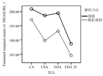
求解柔性流水车间最常用的智能算法是GA[38, 40-42], 较为新颖的是GSA (Gravitational search algorithm)[43-45]和EDA[3, 17], 标识提出的高效EDA为EDA_H.对比这4种算法在规则解码和随机规则解码下的性能, 共进行8组测试, 每组独立运行40次.因文献[17]研究问题与本文一致, EDA算法直接采用其校验的参数, GA和GSA采用第4节的参数检验方法, 结果GA最优参数组合为$P_{size}$=50, 选择概率0.75, 交叉概率0.25, 变异概率0.05, GSA最优参数组合为$P_{size}$=50, 引力系数100, 调整系数为$2\times toc/Zt$, $toc$为当前运行时间, Zt为算法终止的总运行时间.试验均采用Matlab R2010a编程, 运行平台为2.8 GHz的Intel Core i5 CPU和4 GB的RAM个人计算机.用第3.3节中算例, 以Makespan作为评价指标.采用两因素混合设计的方差分析来检验, 组内因素为GA、GSA、EDA和EDA_H 4种算法, 组间因素为规则解码和新解码.方差分析结果展示于表 11~13和图 4.
表 11 四种算法的均值及标准差Table 11 The mean and standard deviation of these four algorithms解码方法 Mean Std. deviation N GA 规则 200.8500 13.46325 40 随机规则 197.2000 13.49112 40 Total 199.0250 13.51696 80 GSA 规则 198.5750 13.51331 40 随机规则 189.7000 12.44928 40 Total 194.1375 13.66020 80 EDA 规则 199.43 13.454 40 随机规则 193.20 12.113 40 Total 196.31 13.100 80 EDA_H 规则 188.68 13.234 40 随机规则 184.42 13.042 40 Total 186.55 13.229 80 表 12 组间因素测试结果Table 12 Test results of between-subjectsSource Square sum df Mean square F Sig. Partial eta squared Intercept 12 044 296.013 1 12 044 296.013 19 397.610 0.000 0.996 Decode 2 645.000 1 2 645.000 4.260 0.042 0.052 Error 48 431.488 78 620.917 - - - 表 13 多元变量测试结果Table 13 Test results of multivariateEffect Value F Hypoth-esis df Error df Sig. Partial eta squared 算法 Pillai's trace 0.882 190.021a 3.000 76.000 0.000 0.882 Wilks' lambda 0.118 190.021a 3.000 76.000 0.000 0.882 Hotelling's trace 7.501 190.021a 3.000 76.000 0.000 0.882 Roy's largest root 7.501 190.021a 3.000 76.000 0.000 0.882 算法加解码 Pillai's trace 0.314 11.617a 3.000 76.000 0.000 0.314 Wilks' lambda 0.686 11.617a 3.000 76.000 0.000 0.314 Hotelling's trace 0.459 11.617a 3.000 76.000 0.000 0.314 Roy's largest root 0.459 11.617a 3.000 76.000 0.000 0.314 表 11为描述统计, 该结果显示4种算法采用新解码的结果都优于原规则解码的结果, 说明新解码方式效果更好; 且表中仅GA算法的方差高于规则解码下的方差, 其他算法的方差均低于规则解码方差, 说明新解码获得最优解的稳定性也较好. 表 12中的显著度为0.042 < 0.050说明两种解码之间存在较显著差异, 由图 4同样可知新解码优于原规则解码. 表 13中的显著度都小于0.050, 说明4种算法性能之间有显著差异, 且算法与解码的交互作用也存在较显著差异, 结合图 4可直观看出, EDA_H性能最好, 其次是GSA, 再其次是EDA, 最后是GA.
5.2 实例测试
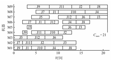
本文利用文献[17]和文献[28]提出的3个FFSP实例, 分别用L1、L2和L3表示, 对比4种算法求解实例的性能差异, 并与文献结果进行对比.采用的终止条件是运行时间10 s, 结果见表 14.通过表中数据可知, EDA_H在求解3个实例时结果好于文献结果, 同时也明显高于其他3种算法, 且更新了文献[17]中的实例L1的最优解, 图 5为EDA_H求得的更新最优解甘特图. EDA_H还更新且获得实例L3的全局最优值, 该值为13与GAMS/Cplex结果一致, 证明获得了全局最优解.
表 14 三个实例在四种算法及原文献中的结果对比Table 14 Comparison for the results of three cases under these four algorithms and original documents次数 文献结果 GA GSA EDA_W EDA_I L1 L2 L3 L1 L2 L3 L1 L2 L3 L1 L2 L3 L1 L2 L3 1 23 297 14 22 298 13.5 22 297 13.5 23 298 13.5 21 297 13 2 24 297 14 22 297 13.5 22 297 13.5 22 297 14 22 297 13 3 23 297 15 22 298 13.5 22 297 13.5 21 300 13.5 21 297 13 4 23 297 14 22 298 13.5 21 298 13.5 22 298 13.5 21 297 13.5 5 23 298 14 22 297 13.5 22 297 13.5 22 297 14 21 297 13 6 23 297 14.5 22 300 13.5 22 298 13.5 21 297 13.5 21 297 13 7 24 297 14 22 298 13.5 21 298 13.5 23 300 14 21 298 13 8 24 298 14.5 22 298 13.5 22 297 13.5 22 197 13.5 21 297 13.5 9 23 298 14 22 298 13.5 22 298 13.5 23 298 13.5 21 297 13 10 24 298 14 22 299 13.5 22 298 13.5 22 298 14 21 297 13 通过表 14的算法对比, 可知EDA_I求解3个实例, 在10次运行中, 任一次求得的结果都不差于其他任何一种算法求解结果, 且绝大部分运行中稳定获得了最优值.说明, EDA_I算法性能最好, 且求解结果也最稳定, 其次是GSA算法.
6. 结论与展望
柔性流水车间是一种具有并行生产设施的流水线车间, 在实际生产中被广泛采用.以最小化Makespan为目标的柔性流水车间调度问题, 其求解性质是NP难.本文在FFSP问题分析基础上构建了求解模型, 并提出了一种高效EDA算法, 该算法采用新解码方式和动态调整概率模型, 同时设计了算法的改进操作, 通过正交实验确定算法参数的最佳组合, 并通过算例测试比较了新算法性能.本文的主要结论如下:
1) 基于机器事件建模思想, 建立0-1混合整数线性规划模型, 采用GAMS/Cplex验证模型有效.
2) 设计FFSP的随机规则解码方式, 通过测试6种概率水平, 确定了概率阈值为0.85.
3) 提出EDA算法动态调整的概率模型, 该概率模型能防止新个体工件的反复无效采样, 提升算法收敛性和搜索效率.
4) 设计带禁忌表的局部搜索和重启机制, 通过正交实验, 确定了合理的算法参数.
算例测试和实例求解结果都表明高效EDA算法在求解质量和稳定性方面优于GA、GSA和EDA_W.
通过本文的研究, 我们发现EDA算法收敛速度快, 但易早熟.因此, 结合新颖高效智能算法, 如GSA求解柔性流水车间调度仍然是一个可行研究领域.特别是结合工程需要, 寻找多约束, 如成组、成批、带No-idle或No-wait约束的柔性流水车间调度, 以及考虑能效或碳排放的FFSP多目标调度是制造行业需重点关注的领域.
-
表 1 解码方法的伪代码和复杂度
Table 1 Pseudo-code and complexity for decoding method
Algorithm 1. Template of decoding O (max{Snlog (n), nMlog (m)}) Input: π as the coding, and πt as the t-th processed job number, P_m as the probability, O (C) j=1 (j is the index of the stages); O (1) Repeat O (max{Snlog (n), nM log (m)}) t=1; O (1) Repeat O (nmjlog (mj)) Randomly generating a number of [0, 1] which is noted as P m; O (1) Calculating the completion time of πt processed on each machine (Tπt, j, k) according to equation (12); O (mj) If P_m≤P_m, the machine of the minimum Tπt, j, k is chosen and is noted as k*; O (mjlog (mj)) Else, a machine is randomly chosen and is noted as k*; O (mjlog (mj)) Setting Eπt, j=Tπt, j, k, Bπt, j=Tπt, j, k* -Pπt, k*; O (1) t + + O (1) Until t=n O (1) Reorganizing the sequence of jobs according to the ascending order of Eπt, j; O (nlog (n)) Updating π as the sequence of jobs; O (n) j + + O (1) Until j=S O (1) Output: Final solution found. O (C)  下载: 导出CSV
表 2 概率矩阵构建与种群更新的伪代码和复杂度
Table 2 Pseudo-code and complexity for constructing probability matrix and updating population
Algorithm 2. Template of construction probability matrix and updating population O (GPsize(n2 -n)/2) Input: Sp as dominant population. Pt.i(g) as the probability matrix; 0(n2) g as the index evolutional generation, g=0; 0(1) Repeat O (GPsize(n2 -n)/2) Determining the values of ISt, il (g) according to Sp; O (n2|Sp|) Calculating Pt, i(g + 1) by equation (13) and setting Pt, i0 (g + 1)=Pt, i(g + 1); 0(n2) l=l; 0(1) Setting I as the sequence of jobs in the individual l; O (n) Repeat O (Psize(n2 -n)/2) t=1; 0(1) Updating the job of individual l which is arranged at position t according to Pt, i0 (g + 1) by the roulette approach; 0(n -1) Noting the job as i* 0(1) Repeat O ((n2-n)/2) I'={i, i ∈ I/i*} O (n -t) Calculating Pt, i0 (g + 1) by equation (14). O (n -t) Dynamically updating Pt', i(g + 1), as Pt', i'(g + 1), O (n -t) t + + O (1) I=[]; I=I'; O (n -t) Updating the job of individual l which is arranged at position t according to (3 + 1) by the roulette approach; O (n -1) Until t==n O (1) l + + O (1) Until l==Psize O (1) Calculating the target values for all of updated individuals by decoding method; O (Psizesnlog (n)) Sequencing the individuals in ascending order of target values; O (Psixesnlog (n)) Selecting the top η % of individuals as sp; O (|sp|) g + + O (1) Until the termination criteria are achieved O (1) Output: Final solution found. O (C)
下载: 导出CSV
表 3 改进概率模型的性能
Table 3 The performance of improved probability model
代数 EDA_I EDA_W 最优值 多样性 时间(s) 最优值 多样性 时间(s) 10代 249.0 0.83 0.93 251.0 0.89 0.97 50代 237.1 0.35 4.78 241.2 0.60 4.80 100代 230.0 0.09 9.71 239.8 0.23 10.02 200代 226.7 0.01 19.38 235.5 0.03 20.72 500代 223.4 0.00 48.31 230.9 0.00 52.60
下载: 导出CSV
表 4 重启操作的正交实验结果
Table 4 Results for orthogonal test of restart operation
参数组合 水平 AVG $Div{\_}h$ G_max Res 1 2 2 1 222.30 2 2 1 2 223.75 3 4 1 1 223.90 4 3 2 1 222.40 5 3 1 3 219.60 6 1 3 1 223.90 7 1 1 1 223.55 8 1 1 2 223.10 9 3 1 1 221.25 10 1 2 3 222.25 11 4 2 2 222.55 12 4 1 3 219.65 13 2 1 1 223.00 14 3 3 2 222.40 15 4 3 1 224.40 16 2 3 3 219.95
下载: 导出CSV
表 5 重启操作的极差表
Table 5 Rang table of restart operation
水平 $Div{\_}\, h$ G_max Res 1 223.200 222.263 223.088 2 222.150 222.375 222.950 3 221.487 222.563 220.338 4 222.625 - - 极差 1.713 0.300 2.750 等级 2 3 1
下载: 导出CSV
表 6 重启操作中三种影响因素的方差分析
Table 6 ANOVA for three factors of restart operation
Source Type Ⅲ sum of squares df Mean square F Sig. Partial eta squared Corrected model 28.553a 7 4.079 4.510 0.025 0.798 Intercept 646 099.042 1 646 099.042 714 322.413 0.000 1.000 $Div{\_}h$ 6.324 3 2.108 2.331 0.151 0.466 G_max 0.240 2 0.120 0.133 0.877 0.032 Res 21.988 2 10.994 12.155 0.004 0.752
下载: 导出CSV
表 7 高效EDA算法各操作复杂度
Table 7 The complexity of efficient EDA
操作名称 复杂度 初始化 O$(nP_{size})$ 评价种群 O$(P_{size} Mn\log (n))$ 选择优势种群并计算概率 O$(n^2SP_{size})$ 按概率生产新种群 O$(n^2P_{size})$ 邻域搜索 O$Mn^{3})$或O$Mn^{2})$ 重启操作 O$(P_{size}${$Mn$log($n))$
下载: 导出CSV
表 8 算法参数正交实验结果
Table 8 Results for orthogonal test of algorithm parameters
参数组合 水平 AVG $Div{\_}h$ G_max Res 1 2 2 4 193.40 2 2 1 2 193.94 3 4 1 4 192.66 4 3 2 1 197.29 5 3 1 3 192.51 6 1 3 4 195.14 7 1 1 1 195.54 8 1 4 2 197.54 9 3 4 4 195.40 10 1 2 3 194.26 11 4 2 2 195.29 12 4 4 3 195.97 13 2 4 1 198.71 14 3 3 2 196.29 15 4 3 1 197.14 16 2 3 3 194.46
下载: 导出CSV
表 9 高效EDA各参数的极差
Table 9 Rang for the parameters of efficient EDA
水平 $Div{\_}\, h$ G_max Res 1 195.620 193.663 197.170 2 195.128 195.060 195.765 3 195.373 195.758 194.300 4 195.265 196.905 194.150 极差 0.492 3.242 3.020 等级 3 1 2
下载: 导出CSV
表 10 高效EDA的三种参数的方差分析
Table 10 ANOVA for three parameters of efficient EDA
Source Type Ⅲ sum of squares df Mean square F Sig. Partial eta squared Corrected model 46.692a 9 5.188 39.490 0.000 0.983 Intercept 610 562.518 1 610 562.518 4 647 478.731 0.000 1.000 $P_{size}$ 0.520 3 0.173 1.320 0.352 0.398 $\eta $ 22.063 3 7.354 55.980 0.000 0.966 a 24.108 3 8.036 61.169 0.000 0.968
下载: 导出CSV
表 11 四种算法的均值及标准差
Table 11 The mean and standard deviation of these four algorithms
解码方法 Mean Std. deviation N GA 规则 200.8500 13.46325 40 随机规则 197.2000 13.49112 40 Total 199.0250 13.51696 80 GSA 规则 198.5750 13.51331 40 随机规则 189.7000 12.44928 40 Total 194.1375 13.66020 80 EDA 规则 199.43 13.454 40 随机规则 193.20 12.113 40 Total 196.31 13.100 80 EDA_H 规则 188.68 13.234 40 随机规则 184.42 13.042 40 Total 186.55 13.229 80
下载: 导出CSV
表 12 组间因素测试结果
Table 12 Test results of between-subjects
Source Square sum df Mean square F Sig. Partial eta squared Intercept 12 044 296.013 1 12 044 296.013 19 397.610 0.000 0.996 Decode 2 645.000 1 2 645.000 4.260 0.042 0.052 Error 48 431.488 78 620.917 - - -
下载: 导出CSV
表 13 多元变量测试结果
Table 13 Test results of multivariate
Effect Value F Hypoth-esis df Error df Sig. Partial eta squared 算法 Pillai's trace 0.882 190.021a 3.000 76.000 0.000 0.882 Wilks' lambda 0.118 190.021a 3.000 76.000 0.000 0.882 Hotelling's trace 7.501 190.021a 3.000 76.000 0.000 0.882 Roy's largest root 7.501 190.021a 3.000 76.000 0.000 0.882 算法加解码 Pillai's trace 0.314 11.617a 3.000 76.000 0.000 0.314 Wilks' lambda 0.686 11.617a 3.000 76.000 0.000 0.314 Hotelling's trace 0.459 11.617a 3.000 76.000 0.000 0.314 Roy's largest root 0.459 11.617a 3.000 76.000 0.000 0.314
下载: 导出CSV
表 14 三个实例在四种算法及原文献中的结果对比
Table 14 Comparison for the results of three cases under these four algorithms and original documents
次数 文献结果 GA GSA EDA_W EDA_I L1 L2 L3 L1 L2 L3 L1 L2 L3 L1 L2 L3 L1 L2 L3 1 23 297 14 22 298 13.5 22 297 13.5 23 298 13.5 21 297 13 2 24 297 14 22 297 13.5 22 297 13.5 22 297 14 22 297 13 3 23 297 15 22 298 13.5 22 297 13.5 21 300 13.5 21 297 13 4 23 297 14 22 298 13.5 21 298 13.5 22 298 13.5 21 297 13.5 5 23 298 14 22 297 13.5 22 297 13.5 22 297 14 21 297 13 6 23 297 14.5 22 300 13.5 22 298 13.5 21 297 13.5 21 297 13 7 24 297 14 22 298 13.5 21 298 13.5 23 300 14 21 298 13 8 24 298 14.5 22 298 13.5 22 297 13.5 22 197 13.5 21 297 13.5 9 23 298 14 22 298 13.5 22 298 13.5 23 298 13.5 21 297 13 10 24 298 14 22 299 13.5 22 298 13.5 22 298 14 21 297 13
下载: 导出CSV
-
[1] Salvador M S. A solution to a special class of flow shop scheduling problems. In:Proceedings of the 1973 Symposium on the Theory of Scheduling and Its Applications. Berlin, Germany:Springer, 1973. 83-92 [2] 李铁克, 苏志雄.炼钢连铸生产调度问题的两阶段遗传算法.中国管理科学, 2009, 17(4):68-74 http://www.cnki.com.cn/Article/CJFDTOTAL-ZGGK200905010.htmLi Tie-Ke, Su Zhi-Xiong. Two-stage genetic algorithm for SM-CC production scheduling. Chinese Journal of Management Science, 2009, 17(4):68-74 http://www.cnki.com.cn/Article/CJFDTOTAL-ZGGK200905010.htm [3] 王圣尧, 王凌, 许烨.求解相同并行机混合流水线车间调度问题的分布估算算法.计算机集成制造系统, 2013, 19(6):1304-1312 http://www.cnki.com.cn/Article/CJFDTOTAL-JSJJ201306018.htmWang Sheng-Yao, Wang Ling, Xu Ye. Estimation of distribution algorithm for solving hybrid flow-shop scheduling problem with identical parallel machine. Computer Integrated Manufacturing Systems, 2013, 19(6):1304-1312 http://www.cnki.com.cn/Article/CJFDTOTAL-JSJJ201306018.htm [4] 王凌, 周刚, 许烨, 金以慧.混合流水线调度研究进展.化工自动化及仪表, 2011, 38(1):1-8, 22 http://www.cnki.com.cn/Article/CJFDTOTAL-HGZD201101002.htmWang Ling, Zhou Gang, Xu Ye, Jin Yi-Hui. Advances in the study on hybrid flow-shop scheduling. Control and Instruments in Chemical Industry, 2011, 38(1):1-8, 22 http://www.cnki.com.cn/Article/CJFDTOTAL-HGZD201101002.htm [5] 王凌, 周刚, 许烨, 王圣尧.求解不相关并行机混合流水线调度问题的人工蜂群算法.控制理论与应用, 2012, 29(12):1551-1557 http://www.cnki.com.cn/Article/CJFDTOTAL-KZLY201212004.htmWang Ling, Zhou Gang, Xu Ye, Wang Sheng-Yao. An artificial bee colony algorithm for solving hybrid flow-shop scheduling problem with unrelated parallel machines. Control Theory & Applications, 2012, 29(12):1551-1557 http://www.cnki.com.cn/Article/CJFDTOTAL-KZLY201212004.htm [6] Graham R L, Lawler E L, Lenstra J K, Kan A H G R. Optimization and approximation in deterministic sequencing and scheduling:a survey. Annals of Discrete Mathematics, 1979, 5:287-326 doi: 10.1016/S0167-5060(08)70356-X [7] Linn R, Zhang W. Hybrid flow shop scheduling:a survey. Computer & Industrial Engineering, 1999, 37(1-2):57-61 http://www.ingentaconnect.com/content/els/03608352/1999/00000037/00000001/art00023 [8] Kis L, Pesch E. A review of exact solution methods for the non-preemptive multiprocessor flowshop problem. European Journal of Operational Research, 2005, 164(3):592-608 doi: 10.1016/j.ejor.2003.12.026 [9] Azizoğlu M, Çakmak E, Kondakci S. A flexible flowshop problem with total flow time minimization. European Journal of Operational Research, 2001, 132(3):528-538 doi: 10.1016/S0377-2217(00)00142-9 [10] Nawaz M, Enscore E E Jr, Ham I. A heuristic algorithm for the m-machine, n-job flow-shop sequencing problem. Omega, 1983, 11(1):91-95 doi: 10.1016/0305-0483(83)90088-9 [11] Palmer D S. Sequencing jobs through a multi-stage process in the minimum total time-a quick method of obtaining a near optimum. Journal of the Operational Research Society, 1965, 16(1):101-107 doi: 10.1057/jors.1965.8 [12] Campbell H G, Dudek R A, Smith M L. A heuristic algorithm for the n job, m machine sequencing problem. Management Science, 1970, 16(10):B630-B637 doi: 10.1287/mnsc.16.10.B630 [13] Ruiz R, Vázquez-Rodríguez J A. The hybrid flow shop scheduling problem. European Journal of Operational Research, 2010, 205(1):1-18 doi: 10.1016/j.ejor.2009.09.024 [14] Shiau D F, Huang Y M. A hybrid two-phase encoding particle swarm optimization for total weighted completion time minimization in proportionate flexible flow shop scheduling. The International Journal of Advanced Manufacturing Technology, 2012, 58(1):339-357 doi: 10.1007/s00170-011-3378-3 [15] Tran T H, Ng K M. A water-flow algorithm for flexible flow shop scheduling with intermediate buffers. Journal of Scheduling, 2011, 14(5):483-500 doi: 10.1007/s10951-010-0205-x [16] 宋代立, 张洁.蚁群算法求解混合流水车间分批调度问题.计算机集成制造系统, 2013, 19(7):1640-1647 http://www.cnki.com.cn/Article/CJFDTOTAL-JSJJ201307024.htmSong Dai-Li, Zhang Jie. Batch scheduling problem of hybrid flow shop based on ant colony algorithm. Computer Integrated Manufacturing Systems, 2013, 19(7):1640-1647 http://www.cnki.com.cn/Article/CJFDTOTAL-JSJJ201307024.htm [17] 王圣尧, 王凌, 许烨, 周刚.求解混合流水车间调度问题的分布估计算法.自动化学报, 2012, 38(3):437-443 doi: 10.3724/SP.J.1004.2012.00437Wang Sheng-Yao, Wang Ling, Xu Ye, Zhou Gang. An estimation of distribution algorithm for solving hybrid flow-shop scheduling problem. Acta Automatica Sinica, 2012, 38(3):437-443 doi: 10.3724/SP.J.1004.2012.00437 [18] Guinet A G P, Solomon M M. Scheduling hybrid flowshops to minimize maximum tardiness or maximum completion time. International Journal of Production Research, 1996, 34(6):1643-1654 doi: 10.1080/00207549608904988 [19] Engin O, Döyen A. A new approach to solve hybrid flow shop scheduling problems by artificial immune system. Future Generation Computer Systems, 2004, 20(6):1083-1095 doi: 10.1016/j.future.2004.03.014 [20] Kahraman C, Engin O, Kaya I, Yilmaz M K. An application of effective genetic algorithms for solving hybrid flow shop scheduling problems. International Journal of Computational Intelligence Systems, 2008, 1(2):134-147 doi: 10.1080/18756891.2008.9727611 [21] Niu Q, Zhou T J, Ma S W. A quantum-inspired immune algorithm for hybrid flow shop with makespan criterion. Journal of Universa1 Computer Science, 2009, 15(4):765-785 https://www.researchgate.net/publication/220349710_A_Quantum-Inspired_Immune_Algorithm_for_Hybrid_Flow_Shop_with_Makespan_Criterion [22] Baluja S. Population-based incremental learning:a method for integrating genetic search based function optimization and competitive learning, Technical Report CMU-CS-94-163, Computer Science Department, Carnegie Mellon University, USA, 1994. [23] Mühlenbein H, Paaß G. From recombination of genes to the estimation of distributions Ⅰ. binary parameters. In:Proceedings of the 4th International Conference on Parallel Problem Solving from Nature. Berlin, Germany:Springer, 1996. 178-187 [24] Larrańaga P, Lozano J A. Estimation of Distribution Algorithms:A New Tool for Evolutionary Computation. Boston, USA:Kluwer Press, 2002. 57-61 [25] 周树德, 孙增圻.分布估计算法综述.自动化学报, 2007, 33(2):113-124 doi: 10.1360/aas-007-0113Zhou Shu-De, Sun Zeng-Qi. A survey on estimation of distribution algorithms. Acta Automatica Sinica, 2007, 33(2):113-124 doi: 10.1360/aas-007-0113 [26] 王圣尧, 王凌, 方晨, 许烨.分布估计算法研究进展.控制与决策, 2012, 27(7):961-966, 974 http://www.cnki.com.cn/Article/CJFDTOTAL-KZYC201207002.htmWang Sheng-Yao, Wang Ling, Fang Chen, Xu Ye. Advances in estimation of distribution algorithms. Control and Decision, 2012, 27(7):961-966, 974 http://www.cnki.com.cn/Article/CJFDTOTAL-KZYC201207002.htm [27] Rabiee M, Rad R S, Mazinani M, Shafaei R. An intelligent hybrid meta-heuristic for solving a case of no-wait two-stage flexible flow shop scheduling problem with unrelated parallel machines. The International Journal of Advanced Manufacturing Technology, 2014, 71(5):1229-1245 https://www.researchgate.net/publication/262686363_An_intelligent_hybrid_meta-heuristic_for_solving_a_case_of_no-wait_two-stage_flexible_flow_shop_scheduling_problem_with_unrelated_parallel_machines?_sg=hC1vVOP0bkPT-eYhm4xL-WBqnnvcOKuG0_yYX3VDOVqmnKCf1gfvUNCxgms3TSRH93CGqFpMCG-oSMaXMYEdmw [28] 张凤超.改进的分布估计算法求解混合流水车间调度问题研究.软件导刊, 2014, 13(8):23-36 http://www.cnki.com.cn/Article/CJFDTOTAL-RJDK201408010.htmZhang Feng-Chao. An improved estimation of distribution algorithm to solve the hybrid flow shop scheduling problem. Software Guide, 2014, 13(8):23-36 http://www.cnki.com.cn/Article/CJFDTOTAL-RJDK201408010.htm [29] Shaik M A, Floudas C A. Unit-specific event-based continuous-time approach for short-term scheduling of batch plants using RTN framework. Computers & Chemical Engineering, 2008, 32(1-2):260-274 https://www.researchgate.net/publication/223556750_Unit-specific_event-based_continuous-time_approach_for_short-term_scheduling_of_batch_plants_using_RTN_framework [30] Li J, Floudas C A. Optimal event point determination for short-term scheduling of multipurpose batch plants via unit-specific event-based continuous-time approaches. Industrial & Engineering Chemistry Research, 2010, 49(16):7446-7469 https://www.researchgate.net/publication/231391276_Optimal_Event_Point_Determination_for_Short-Term_Scheduling_of_Multipurpose_Batch_Plants_via_Unit-Specific_Event-Based_Continuous-Time_Approaches [31] Li J, Xiao X, Tang Q H, Floudas C A. Production scheduling of a large-scale steelmaking continuous casting process via unit-specific event-based continuous-time models:short-term and medium-term scheduling. Industrial & Engineering Chemistry Research, 2012, 51(21):7300-7319 https://www.researchgate.net/publication/263954240_Production_Scheduling_of_a_Large-Scale_Steelmaking_Continuous_Casting_Process_via_Unit-Specific_Event-Based_Continuous-Time_Models_Short-Term_and_Medium-Term_Scheduling [32] 陈荣秋.生产计划与控制:概念、方法与系统.武汉:华中理工大学出版社, 1995. 48Chen Rong-Qiu. Production Planning and Control:Concept, Method and System. Wuhan:Huazhong University of Technology Press, 1995. 48 [33] Shaffer C A[著], 张铭, 刘晓丹等[译].数据结构与算法分析(C++版) (第3版).北京:电子工业出版社, 2013. 31Shaffer C A[Author], Zhang Ming, Liu Xiao-Dan, et al[Translator]. Data structure and Algorithm Analysis in C++(Third edition). Beijing:Publishing House of Electronics Industry, 2013. 31 [34] Pan Q K, Ruiz R. An estimation of distribution algorithm for lot-streaming flow shop problems with setup times. Omega, 2012, 40(2):166-180 doi: 10.1016/j.omega.2011.05.002 [35] 屈国强.瓶颈指向的启发式算法求解混合流水车间调度问题.信息与控制, 2012, 41(4):514-521, 528 http://www.cnki.com.cn/Article/CJFDTOTAL-XXYK201204019.htmQu Guo-Qiang. Bottleneck focused heuristic algorithm for hybrid flow shop scheduling problem. Information and Control, 2012, 41(4):514-521, 528 http://www.cnki.com.cn/Article/CJFDTOTAL-XXYK201204019.htm [36] 潘全科, 高亮, 李新宇.流水车间调度及其优化算法.武汉:华中科技大学出版社, 2013. 97-101Pan Quan-Ke, Gao Liang, Li Xin-Yu. Flow Shop Scheduling and Optimization Algorithms. Wuhan:Huazhong University of Technology Press, 2013. 97-101 [37] Pan Q K, Ruiz R. An effective iterated greedy algorithm for the mixed no-idle permutation flowshop scheduling problem. Omega, 2014, 44:41-50 doi: 10.1016/j.omega.2013.10.002 [38] Vallada E, Ruiz R. Genetic algorithms with path relinking for the minimum tardiness permutation flowshop problem. Omega, 2010, 38(1-2):57-67 doi: 10.1016/j.omega.2009.04.002 [39] Wineberg M, Oppacher F. The underlying similarity of diversity measures used in evolutionary computation. Genetic and Evolutionary Computation. Berlin, Heidelberg:Springer, 2003. 1493-1504 [40] Ruiz R, Maroto C, Alcaraz J. Two new robust genetic algorithms for the flowshop scheduling problem. Omega, 2006, 34(5):461-476 doi: 10.1016/j.omega.2004.12.006 [41] 王凌.车间调度及其遗传算法.北京:清华大学出版社, 2003. 127Wang Ling. Shop Scheduling with Genetic Algorithms. Beijing:Tsinghua University Press, 2003. 127 [42] Ruiz R, Maroto C. A genetic algorithm for hybrid flowshops with sequence dependent setup times and machine eligibility. European Journal of Operational Research, 2006, 169(3):781-800 doi: 10.1016/j.ejor.2004.06.038 [43] Han X H, Chang X M. A chaotic digital secure communication based on a modified gravitational search algorithm filter. Information Sciences, 2012, 208:14-27 doi: 10.1016/j.ins.2012.04.039 [44] Bahrololoum A, Nezamabadi-Pour H, Bahrololoum H, Saeed M. A prototype classifier based on gravitational search algorithm. Applied Soft Computing, 2012, 12(2):819-825 doi: 10.1016/j.asoc.2011.10.008 [45] 谷文祥, 李向涛, 朱磊, 周俊萍, 胡艳梅.求解流水线调度问题的万有引力搜索算法.智能系统学报, 2010, 5(5):411-418 http://www.cnki.com.cn/Article/CJFDTOTAL-ZNXT201005005.htmGu Wen-Xiang, Li Xiang-Tao, Zhu Lei, Zhou Jun-Ping, Hu Yan-Mei. A gravitational search algorithm for flow shop scheduling. CAAI Transactions on Intelligent Systems, 2010, 5(5):411-418 http://www.cnki.com.cn/Article/CJFDTOTAL-ZNXT201005005.htm 期刊类型引用(19)
1. 周伟,丁雪莹,谢志强. 考虑柔性设备加工能力的综合调度算法. 华南师范大学学报(自然科学版). 2024(02): 110-118 .  百度学术
百度学术2. 郑堃,练志伟,顾新艳,朱长建,徐慧,冯雪晴. 采用改进两点交叉算子的改进自适应遗传算法求解不相关并行机混合流水车间调度问题. 中国机械工程. 2023(14): 1647-1658+1671 . 百度学术3. 李瑞,龚文引. 改进的基于分解的多目标进化算法求解双目标模糊柔性作业车间调度问题. 控制理论与应用. 2022(01): 31-40 . 百度学术4. 张彪,孟磊磊,桑红燕,卢超. 多目标变分批混合流水车间调度算法自动设计. 计算机集成制造系统. 2022(11): 3403-3420 . 百度学术5. 轩华,郑倩倩,李冰. 带不相关并行机的阻塞FFP的混合遗传算法. 计算机工程与设计. 2021(04): 949-956 . 百度学术6. 罗浩嘉,潘大志. 求解柔性车间调度问题的双层编码离散布谷鸟算法. 计算机与数字工程. 2021(07): 1281-1285+1301 . 百度学术7. 牟云,阎春平,刘艺繁,孙雷. 考虑能耗和完工时间的柔性流水车间调度方法. 制造业自动化. 2021(10): 45-52+74 . 百度学术8. 时维国,宋存利. 求解混合流水车间调度问题的改进灰狼算法. 计算机集成制造系统. 2021(11): 3196-3208 . 百度学术9. 杜士卿,朱光宇,徐文婕. 最佳觅食算法求解多目标混合流水车间调度问题. 福州大学学报(自然科学版). 2020(03): 325-332 . 百度学术10. 宫敬程,庄存波,刘检华,何永熹,曹远冲. 基于磷虾群-禁忌算法的复杂产品装配调度问题. 现代制造工程. 2020(09): 32-39+61 . 百度学术11. 罗函明,罗天洪,吴晓东,陈科百. 求解混合流水车间调度问题的离散布谷鸟算法. 计算机工程与应用. 2020(22): 264-271 . 百度学术12. 宁桂英,曹敦虔. 混合差分进化算法求解柔性作业车间调度问题. 佳木斯大学学报(自然科学版). 2020(06): 101-106+122 . 百度学术13. 宋存利. 求解混合流水车间调度的改进贪婪遗传算法. 系统工程与电子技术. 2019(05): 1079-1086 . 百度学术14. 杨晓林,胡蓉,钱斌,吴丽萍. 增强分布估计算法求解低碳分布式流水线调度. 控制理论与应用. 2019(05): 803-815 . 百度学术15. 顾蕾. 求解静态流水车间调度的改进遗传算法. 电子技术与软件工程. 2019(15): 118-119 . 百度学术16. 任彩乐,杨旭东,张超勇,孟磊磊,洪辉,余俊. 面向节能的混合流水车间调度问题建模与优化. 计算机集成制造系统. 2019(08): 1965-1980 . 百度学术17. 庄存波,熊辉,刘检华,唐承统. 一种改进离散磷虾群的复杂产品装配调度算法. 兵工学报. 2018(08): 1590-1600 . 百度学术18. 吕聪,魏康林. 柔性车间调度问题的协作混合帝国算法. 计算机应用. 2018(07): 1882-1887 . 百度学术19. 张贵军,王文,周晓根,王柳静. 基于动态策略的差分进化柔性车间优化调度. 计算机科学. 2018(10): 240-245 . 百度学术其他类型引用(31)
-

 下载:
下载:


计量
- 文章访问数: 2842
- HTML全文浏览量: 402
- PDF下载量: 1234
- 被引次数: 50
