

-
摘要: 针对低资源训练数据条件下深层神经网络(Deep neural network,DNN)特征声学建模性能急剧下降的问题,提出两种适合于低资源语音识别的深层神经网络特征提取方法.首先基于隐含层共享训练的网络结构,借助资源较为丰富的语料实现对深层瓶颈神经网络的辅助训练,针对BN层位于共享层的特点,引入Dropout,Maxout,Rectified linear units等技术改善多流训练样本分布不规律导致的过拟合问题,同时缩小网络参数规模、降低训练耗时;其次为了改善深层神经网络特征提取方法,提出一种基于凸非负矩阵分解(Convex-non-negative matrix factorization,CNMF)算法的低维高层特征提取技术,通过对网络的权值矩阵分解得到基矩阵作为特征层的权值矩阵,然后从该层提取一种新的低维特征.基于Vystadial 2013的1小时低资源捷克语训练语料的实验表明,在26.7小时的英语语料辅助训练下,当使用Dropout和Rectified linear units时,识别率相对基线系统提升7.0%;当使用Dropout和Maxout时,识别率相对基线系统提升了12.6%,且网络参数数量相对其他系统降低了62.7%,训练时间降低了25%.而基于矩阵分解的低维特征在单语言训练和辅助训练的两种情况下都取得了优于瓶颈特征(Bottleneck features,BNF)的识别率,且在辅助训练的情况下优于深层神经网络隐马尔科夫识别系统,提升幅度从0.8%~3.4%不等.Abstract: To alleviate the performance degradation that deep neural network (DNN) based features suffer from transcribed training data is insufficient, two deep neural network based feature extraction approaches to low-resource speech recognition are proposed. Firstly, some high-resource corpuses are used to help train a bottleneck deep neural network using a shared-hidden-layer network structure and dropout, maxout, and rectified linear units methods are exploited in order to enhance the training effect and reduce the number of network parameters, so that the overfitting problem by irregular distributions of multi-stream training samples can be solved and multilingual training time can be reduced. Secondly, a convex-non-negative matrix factorization (CNMF) based low-dimensional high-level feature extraction approach is proposed. The weight matrix of hidden layer is factorized to obtain the basis matrix as the weight matrix of the newly formed feature-layer, from which a new type of feature is extracted. Experiments on 1 hour's Vystadial 2013 Czech low-resource training data show that with the help of 26.7 hours' English training data, the recognition system obtains a 7.0% relative word error rate reduction from the baseline system when dropout and rectified linear units are applied, and obtains a 12.6% relative word error rate reduction while reduces 62.7% relative network parameters and 25% training time as compared to other proposed systems when dropout and maxout are applied. Matrix factorization based features perform better than bottleneck features (BNF) in both low-resource monolingual and multilingual training situations. They also gain better word accuracies than the state-of-art deep neural network hidden Markov models hybrid systems, by from 0.8% to 3.4%.1) 本文责任编委 贾珈
-
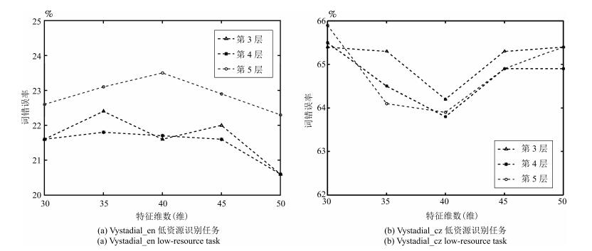
图 4 不同分解参数下基于CNMF的低维特征词错误率
Fig. 4 WER of CNMF based low-dimensional features under difierent factorization parameters
表 1 不同训练方法下BNF的WER (%)
Table 1 WER of BNF based on different training methods (%)
训练方案 WER DNN参数数量(MB) 单语言BNF 67.42 3.57 SHL + BNF 63.25 8.34 SHL + Dropout + Maxout + BNF 58.95 3.11 SHL + Dropout + ReLU + BNF 62.74 8.34  下载: 导出CSV
表 2 不同dropout和maxout参数下的WER (%)
Table 2 WER under difierent dropout and maxout parameters (%)
Dropout-maxout参数 HDF = 0.1 HDF = 0.1 HDF = 0.2 HDF = 0.2 HDF = 0.3 HDF = 0.3 BN-DF = 0 BN-DF = 0.1 BN-DF = 0 BN-DF = 0.2 BN-DF = 0 BN-DF = 0.3 Pooling尺寸: 512×2 (40×2) 62.11 60.77 61.89 Pooling尺寸: 342×3 (40×3) 59.72 61.14 58.95 60.32 60.13 61.5 Pooling尺寸: 256×4 (40×4) 61.23 60.36 61.84
下载: 导出CSV
表 3 基于单语言训练时各特征的识别性能WER (%)
Table 3 Recognition performance WER each type of feature based on monolingual training (%)
识别任务 BNF CNMF低维特征 SVD低维特征 低资源Vystadial_en 21.6 20.6 21.51 低资源Vystadial_cz 64.8 63.76 64.43
下载: 导出CSV
表 4 基于SHL多语言训练的CNMF低维特征的WER (%)
Table 4 WER of SHL multilingual training CNMF based low-dimensional features (%)
CNMF特征提取方案 第3层 第4层 第5层 Sigmoid + 40维分解 64.27 64.94 64.71 Sigmoid + 50维分解 63.86 63.81 64.99 Dropout + Maxout + 40维分解 60.33 60.13 59.59 Dropout + Maxout + 50维分解 59.59 59.12 59.95 Dropout + ReLU + 40维分解 63.71 61.59 61.28 Dropout + ReLU + 50维分解 62.15 60.26 61.84
下载: 导出CSV
表 5 BNF与CNMF低维特征的GMM tandem系统WER (%)
Table 5 WER of BNF and CNMF based low-dimensional features on GMM tandem system (%)
实验配置 BNF CNMF低维特征 Vystadial_en (单语言fMLLR) + Sigmoid-DNN 21.6 20.6 Vystadial_cz (单语言fMLLR) + Sigmoid-DNN 64.8 63.76 Vystadial_cz (单语言fbanks) + Sigmoid-DNN 63.25 63.81 Vystadial_cz (单语言fbanks) + Dropout-maxout-DNN 58.95 59.12 Vystadial_cz (单语言fbanks) + Dropout-ReLU-DNN 62.74 60.26
下载: 导出CSV
表 6 基于SHL多语言训练时SGMM tandem系统和DNN-HMM系统的WER (%)
Table 6 WER of SGMM tandem systems and DNN-HMM hybrid systems based on SHL multilingual training (%)
DNN隐含层结构 BNF CNMF低维特征 DNN-HMM 5层1 024 (BN: 40) 63.15 61.79 63.94 Sigmoid 3层1 024 (BN: 40) 63.09 61.85 63.99 3层512 (BN: 40) 63.5 61.84 63.96 5层342 (*3, BN: 40) 58.03 57.8 58.24 Dropout + Maxout 3层342 (*3, BN: 40) 60.61 60.4 63.99 3层171 (*3, BN: 40) 62.61 64.72 68.77 5层1 024 (BN: 40) 60.72 58.82 59.57 Dropout + ReLU 3层1 024 (BN: 40) 64.35 59.16 59.92 3层512 (BN: 40) 63.43 61.68 62.2
下载: 导出CSV
-
[1] Thomas S. Data-driven Neural Network Based Feature Front-ends for Automatic Speech Recognition[Ph.D. dissertation], Johns Hopkins University, Baltimore, USA, 2012. [2] Grézl F, Karaát M, Kontár S, Černocký J. Probabilistic and bottle-neck features for LVCSR of meetings. In:Proceedings of the 2007 International Conference on Acoustics, Speech and Signal Processing (ICASSP). Hawaii, USA:IEEE, 2007. 757-760 [3] Yu D, Seltzer M L. Improved bottleneck features using pretrained deep neural networks. In:Proceedings of the 12th Annual Conference of the International Speech Communication Association (INTERSPEECH). Florence, Italy:Curran Associates, Inc., 2011. 237-240 [4] Bao Y B, Jiang H, Dai L R, Liu R. Incoherent training of deep neural networks to de-correlate bottleneck features for speech recognition. In:Proceedings of the 2013 International Conference on Acoustics, Speech, and Signal Processing (ICASSP). Vancouver, BC, Canada:IEEE, 2013. 6980-6984 [5] Hinton G E, Deng L, Yu D, Dahl D E, Mohamed A R, Jaitly N, Senior A, Vanhoucke V, Nguyen P, Sainath T N, Kingsbury B. Deep neural networks for acoustic modeling in speech recognition:the shared views of four research groups. IEEE Signal Processing Magazine, 2012, 29 (6):82-97 doi: 10.1109/MSP.2012.2205597 [6] Lal P, King S. Cross-lingual automatic speech recognition using tandem features. IEEE Transactions on Audio, Speech, and Language Processing, 2013, 21 (12):2506-2515 doi: 10.1109/TASL.2013.2277932 [7] Veselý K, Karafiát M, Grézl F, Janda M, Egorova E. The language-independent bottleneck features. In:Proceedings of the 2012 IEEE Spoken Language Technology Workshop (SLT). Miami, Florida, USA:IEEE, 2012. 336-341 [8] Tüske Z, Pinto J, Willett D, Schlüter R. Investigation on cross-and multilingual MLP features under matched and mismatched acoustical conditions. In:Proceedings of the 2013 IEEE International Conference on Acoustics, Speech, and Signal Processing (ICASSP). Vancouver, BC, Canada:IEEE, 2013. 7349-7353 [9] Gehring J, Miao Y J, Metze F, Waibel A. Extracting deep bottleneck features using stacked auto-encoders. In:Proceedings of the 2013 IEEE International Conference on Acoustics, Speech, and Signal Processing (ICASSP). Vancouver, BC, Canada:IEEE, 2013. 3377-3381 [10] Miao Y J, Metze F. Improving language-universal feature extraction with deep maxout and convolutional neural networks. In:Proceedings of the 15th Annual Conference of the International Speech Communication Association (INTERSPEECH). Singapore:International Speech Communication Association, 2014. 800-804 [11] Huang J T, Li J Y, Dong Y, Deng L, Gong Y F. Cross-language knowledge transfer using multilingual deep neural network with shared hidden layers. In:Proceedings of the 2013 IEEE International Conference on Acoustics, Speech, and Signal Processing (ICASSP). Vancouver, BC, Canada:IEEE, 2013. 7304-7308 [12] Hinton G E, Srivastava N, Krizhevsky A, Sutskever I, Salakhutdinov R R. Improving neural networks by preventing co-adaptation of feature detectors. Computer Science, 2012, 3 (4):212-223 [13] Goodfellow I J, Warde-Farley D, Mirza M, Courville A, Bengio Y. Maxout networks. In:Proceedings of the 30th International Conference on Machine Learning (ICML). Atlanta, GA, USA:ICML, 2013:1319-1327 [14] Zeiler M D, Ranzato M, Monga R, Mao M, Yang K, Le Q V, Nguyen P, Senior A, Vanhoucke V, Dean J, Hinton G H. On rectified linear units for speech processing. In:Proceedings of the 2013 IEEE International Conference on Acoustics, Speech, and Signal Processing (ICASSP). Vancouver, BC, Canada:IEEE, 2013. 3517-3521 [15] Dahl G E, Yu D, Deng L, Acero A. Context-dependent pre-trained deep neural networks for large-vocabulary speech recognition. IEEE Transactions on Audio, Speech, and Language Processing, 2012, 20 (1):30-42 doi: 10.1109/TASL.2011.2134090 [16] Lee D D, Seung H S. Learning the parts of objects by non-negative matrix factorization. Nature, 1999, 401 (6755):788-791 doi: 10.1038/44565 [17] Wilson K W, Raj B, Smaragdis P, Divakaran A. Speech denoising using nonnegative matrix factorization with priors. In:Proceedings of the 2008 International Conference on Acoustics, Speech, and Signal Processing (ICASSP). Las Vegas, NV, USA:IEEE, 2008. 4029-4032 [18] Mohammadiha N. Speech Enhancement Using Nonnegative Matrix Factorization and Hidden Markov Models[Ph.D. dissertation], KTH Royal Institute of Technology, Stockholm, Sweden, 2013. [19] Ding C H Q, Li T, Jordan M I. Convex and semi-nonnegative matrix factorizations. IEEE Transactions on Pattern Analysis and Machine Intelligence, 2010, 32 (1):45-55 doi: 10.1109/TPAMI.2008.277 [20] Price P, Fisher W, Bernstein J, Pallett D. Resource management RM12.0[Online], available:https://catalog.ldc.upenn.edu/LDC93S3B, May 16, 2015 [21] Garofolo J, Lamel L, Fisher W, Fiscus J, Pallett D, Dahlgren N, Zue V. TIMIT acoustic-phonetic continuous speech corpus[Online], available:https://catalog.ldc.upenn.edu/LDC93S1, May 16, 2015 [22] Korvas M, Plátek O, Dušek O, Žćilka L, Jurčíček F. Vystadial 2013 English data[Online], available:https://lindat.mff.cuni.cz/repository/xmlui/handle/11858/00-097C-0000-0023-4671-4, May 17, 2015 [23] Korvas M, Plátek O, Dušek O, Žćilka L, Jurčíček F. Vystadial 2013 Czech data[Online], available:https://lindat.mff.cuni.cz/repository/xmlui/handle/11858/00-097C-0000-0023-4670-6?show=full, May 17, 2015 [24] Povey D, Ghoshal A, Boulianne G, Burget L, Glembek O, Goel N, Hannemann M, Motlicek P, Qian Y M, Schwarz P, Silovsky J, Stemmer G, Vesely K. The Kaldi speech recognition toolkit. In:Proceedings of the 2011 IEEE Workshop on Automatic Speech Recognition and Understanding (ASRU). Hawaii, USA:IEEE Signal Processing Society, 2011. 1-4 [25] Miao Y J. Kaldi + PDNN:Building DNN-based ASR Systems with Kaldi and PDNN. arXiv preprint arXiv:1401. 6984, 2014. [26] Thurau C. Python matrix factorization module[Online], available:https://pypi.python.org/pypi/PyMF/0.1.9, September 25, 2015 [27] Sainath T N, Kingsbury B, Ramabhadran B. Auto-encoder bottleneck features using deep belief networks. In:Proceedings of the 2012 IEEE International Conference on Acoustics, Speech, and Signal Processing (ICASSP). Kyoto, Japan:IEEE, 2012. 4153-4156 [28] Miao Y J, Metze F. Improving low-resource CD-DNN-HMM using dropout and multilingual DNN training. In:Proceedings of the 12th Annual Conference of the International Speech Communication Association (INTERSPEECH). Lyon, France:Interspeech, 2013. 2237-2241 [29] Miao Y J, Metze F, Rawat S. Deep maxout networks for low-resource speech recognition. In:Proceedings of the 2013 IEEE Workshop on Automatic Speech Recognition and Understanding (ASRU). Olomouc, Czech:IEEE, 2013. 398-403 [30] Povey D, Burget L, Agarwal M, Akyazi P, Feng K, Ghoshal A, Glembek O, Goel N K, Karafiát M, Rastrow A, Rastrow R C, Schwarz P, Thomas S. Subspace Gaussian mixture models for speech recognition. In:Proceedings of the 2010 IEEE International Conference on Acoustics, Speech, and Signal Processing (ICASSP). Texas, USA:IEEE, 2010. 4330-4333 [31] 吴蔚澜, 蔡猛, 田垚, 杨晓昊, 陈振锋, 刘加, 夏善红.低数据资源条件下基于Bottleneck特征与SGMM模型的语音识别系统.中国科学院大学学报, 2015, 32 (1):97-102 http://www.cnki.com.cn/Article/CJFDTOTAL-ZKYB201501017.htmWu Wei-Lan, Cai Meng, Tian Yao, Yang Xiao-Hao, Chen Zhen-Feng, Liu Jia, Xia Shan-Hong. Bottleneck features and subspace Gaussian mixture models for low-resource speech recognition. Journal of University of Chinese Academy of Sciences, 2015, 32 (1):97-102 http://www.cnki.com.cn/Article/CJFDTOTAL-ZKYB201501017.htm -

 下载:
下载:


计量
- 文章访问数: 3191
- HTML全文浏览量: 526
- PDF下载量: 1044
- 被引次数: 0
