

Finite Time Formation Control for Multiple Vehicles Based on Pontryagin's Minimum Principle
-
摘要: 研究基于庞特里亚金极小值原理的多运载体有限时间编队问题.运载体刻画为欧氏群切丛上演化的全驱动刚体动力学模型.编队机动时间以及队形的几何结构是由编队任务指定的.对于期望的队形,首先利用庞特里亚金最小值原理给出了开环最优控制.为了克服开环控制对扰动的敏感性并增加针对初始条件不确定性摄动的鲁棒性,在假定运载体间通讯为全联通的模式下,通过反馈将系统当前状态作为初始状态,当前时刻作为初始时刻,进一步将开环控制律转化为闭环形式.为了验证所得结果,给出了平面及空间运载体编队的仿真算例.Abstract: The paper studies the problem of finite time formation control for multiple vehicles based on Pontryagin's minimum principle. The vehicle is modeled as a fully actuated rigid body with the dynamics evolving on the tangent bundle of Euclidean group. Both the formation maneuver time and the geometric structure of the formation are specified by the formation task. For the required formation, an open loop optimal control law is derived by using Pontryagin's minimum principle. In order to overcome the sensitivity of the open-loop control to the disturbance and increase the robustness of the control law to the initial perturbation, the open loop control law is converted to the closed loop form. This is done by feeding the current state back and initializing the control law at the current time, under the assumption that the mode of communication between the vehicles is all-to-all. For demonstration of the result, some numerical examples of formations for both planar and spacial vehicles are included.
-
Key words:
- Finite time formation control /
- consensus /
- multiple vehicles /
- minimum principle
-
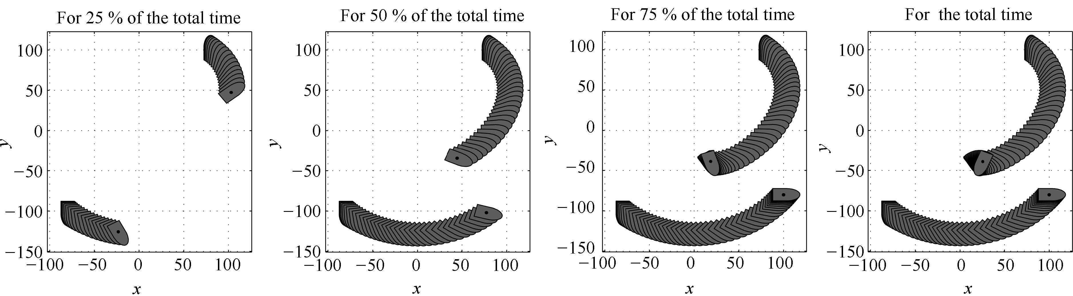
图 1 两运载体的质心位置、姿态演化轨迹(第3图为$t =t_f$时的质心位置、姿态演化轨迹.
Fig. 1 The evolution trajectories of position and attitude of the two vehicles (The 3rd figure are the evolution trajectories of position and attitude at $t = t_f$.

图 2 取得一致性过程中两运载体的时间行为(从上到下: 空间坐标系下的位形(质心位置与姿态角);相对于第一个运载体刚体坐标系下的相对位形; 刚体坐标系下的速度;刚体坐标系下的控制. 从左到右: 相应变量的 $x$-轴坐标;$y$-轴坐标; 姿态角$\theta$轴坐标.
Fig. 2 The time behaviors of the two vehicles during the process of achieving consensus (From top to down: configuration(position and attitude angle) in the space frame; relative configuration with respect to the body frame of first vehicle;velocity in the body frame; control in the body frame. From left to right: the coordinates of the corresponding quantity in $x$-axis,$y$-axis,and attitude angle $\theta$.

图 3 两运载体的质心位置、姿态演化轨迹(左下角为$t = t_f$时的质心位置、姿态演化轨迹.
Fig. 3 The evolution trajectories of position and attitude of the two vehicles (The figure on the bottom left are the evolution trajectories of position and attitude at $t = t_f$.)

图 4 取得一致性过程中两运载体的时间行为(从上到下:空间坐标系下的位形(质心位置与姿态角);相对于第一个运载体刚体坐标系下的相对位形;刚体坐标系下的速度; 刚体坐标系下的控制. 从左到右: 相应变量的$x$-轴坐标; $y$-轴坐标; 姿态角$\theta$轴坐标
Fig. 4 The time behaviors of the two vehicles during the process of achieving consensus (From the top down: configuration(position and attitude angle) in the space frame; relative configuration with respect to the body frame of first vehicle;velocity in the body frame; control in the body frame. From left to right: the coordinates of the corresponding quantity in $x$-axis,$y$-axis,and attitude angle $\theta$.

图 5 两运载体的质心位置、姿态演化轨迹(左下角为$t = t_f$时的质心位置、姿态演化轨迹.
Fig. 5 The evolution trajectories of position and attitude of the two vehicles (The figure on the bottom left are the evolution trajectories of position and attitude at $t = t_f$.
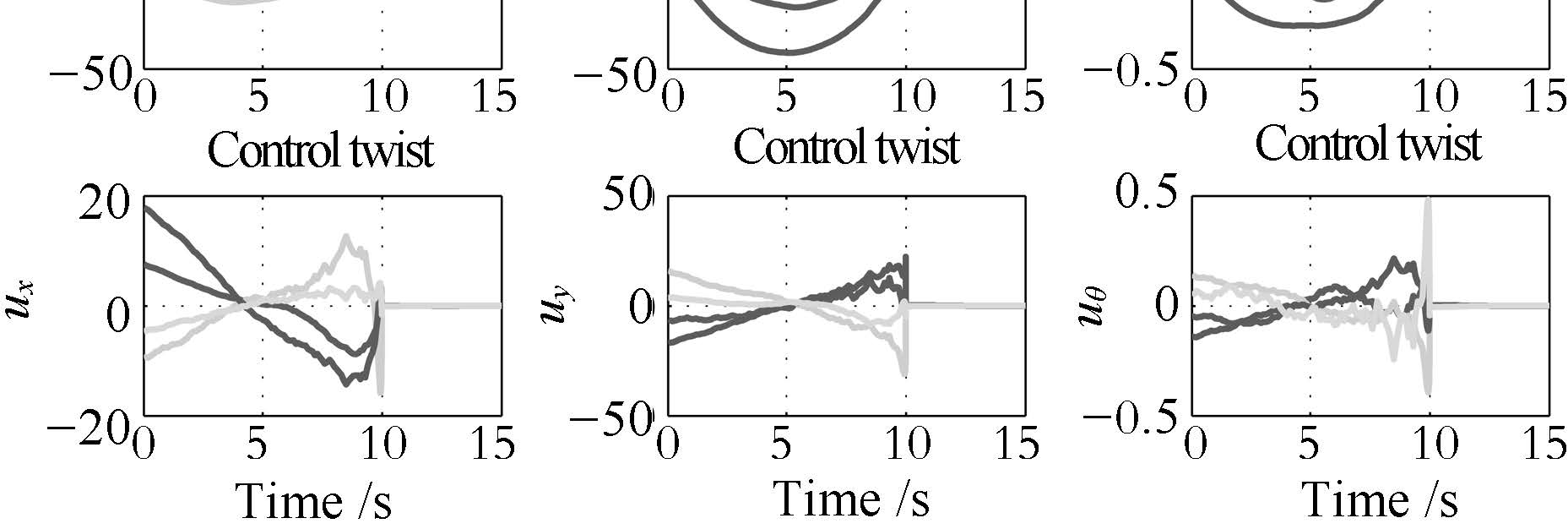
图 6 取得一致性过程中两运载体的时间行为(从上到下:空间坐标系下的位形(质心位置与姿态角);相对于第一个运载体刚体坐标系下的相对位形;刚体坐标系下的速度; 刚体坐标系下的控制. 从左到右: 相应变量的$x$-轴坐标; $y$-轴坐标; 姿态角$\theta$轴坐标.
Fig. 6 The time behaviors of the two vehicles during the process of achieving consensus (From top to down: configuration(position and attitude angle) in the space frame; relative configuration with respect to the body frame of first vehicle;velocity in the body frame; control in the body frame. From left to right: the coordinates of the corresponding quantity in $x$-axis,$y$-axis,and attitude angle $\theta$.

图 7 两运载体的质心位置、姿态演化轨迹(左上角为$t = t_f$时的质心位置、姿态演化轨迹
Fig. 7 The evolution trajectories of position and attitude of the two vehicles (The figure on the top left are the evolution trajectories of position and attitude at $t = t_f$.)

图 8 取得一致性过程中两运载体的时间行为(从上到下: 空间坐标系下的位形(质心位置与姿态角);相对于第一个运载体刚体坐标系下的相对位形; 刚体坐标系下的速度;刚体坐标系下的控制. 从左到右: 相应变量的 $x$-轴坐标;$y$-轴坐标; 姿态角$\theta$轴坐标.
Fig. 8 The time behaviors of the two vehicles during the process of achieving consensus (From the top down: configuration(position and attitude angle) in the space frame; relative configuration with respect to the body frame of first vehicle;velocity in the body frame; control in the body frame. From left to right: the coordinates of the corresponding quantity in$x$-axis,$y$-axis,and attitude angle $\theta$.)

图 9 系统状态的时间行为 (从上到下:空间坐标系下的欧拉角; 质心位置以及刚体坐标系下的旋转速度和平移速度.从左到右: 相应变量的$x$-轴坐标; $y$-轴坐标;$z$-轴坐标.
Fig. 9 Time behaviors of system$'$s states (From the top down: Euler angle; position in the space frame; rotation velocity in the body frame; translation velocity in the body frame. From left to right: the coordinates of the corresponding quantity in$x$-axis,$y$-axis,and $z$-axis.

图 10 系统相对于第一个运载体刚体坐标系下的相对状态 (从上到下: 相对欧拉角;相对位置; 相对旋转速度; 相对平移速度. 从左到右:相应变量的$x$-轴坐标; $y$-轴坐标; $z$-轴坐标.
Fig. 10 Time behaviors of system$'$s relative states with respect to the body coordinate of the first agent (From top to down: relative Euler angle; relative position; relative rotation velocity; relative translation velocity. From left to right: the coordinates of the corresponding quantity in $x$-axis,$y$-axis,and$z$-axis.)

图 11 在刚体坐标系下的控制时间行为 (从上到下:广义力矩; 广义力. 从左到右: 相应变量的$x$-轴坐标;$y$-轴坐标; $z$-轴坐标.)
Fig. 11 Time behaviors of system$'$s control in the body coordinate (From top to down: generalized torque; and generalized force. From left to right: the coordinates of the corresponding quantity in $x$-axis,$y$-axis,and $z$-axis.)

图 12 空间四运载体质心位置、姿态演化轨迹
Fig. 12 The evolution trajectories of position and attitude of the four vehicles
表 1 运载体的初始位形
Table 1 Initial configurations of agents
序号 1 2 $x(0) $ 80 $-80$ $y(0) $ 100 $-100$ $\theta(0) $ $\dfrac{\pi}{2}$ $-\dfrac{\pi}{2}$ 初始位形是由空间坐标系下的质心位置坐标$(x,y)$ 和姿态角$\theta$给出.  下载: 导出CSV
表 2 运载体的初始位形
Table 2 Initial configurations of agents
序号 1 2 3 4 $x(0) $ 100 -100 -100 100 $y(0) $ 100 -100 100 -100 $\theta(0) $ 0 $-\pi$ ${\pi}/{2}$ $-{\pi}/{2}$ 初始位形是由空间坐标系下的质心位置坐标$(x,y)$ 和姿态角$\theta$给出.
下载: 导出CSV
表 3 终端时刻相对位形
Table 3 Relative configurations at final time
相对指标$(1i)$ (11) (12) (13) (14) $x_{1i}(t_f)$ 0 -40 -40 -80 $y_{1i}(t_f)$ 0 -40 40 0 $\theta_{1i}(t_f)$ 0 0 0 0 队形由相对于第一运载体刚体坐标系的相对质心位置坐标$(x_{1i},y_{1i})$和相对姿态角$\theta_{1i}$给出.
下载: 导出CSV
表 4 运载体的初始位形和初始速度
Table 4 Initial configurations and initial velocities of vehicles
序号 1 2 3 4 $x(0) $ 100 -100 -100 100 $y(0) $ 100 -100 100 -100 $\theta(0) $ 0 $-\pi$ ${\pi}/{2}$ $-{\pi}/{2}$ $v_x(0) $ 15 10 7 5 $v_y(0) $ 0 0 0 0 $v_{\theta}(0) $ 0.05 0.02 0.08 0.05 初始位形由空间坐标系下的质心位置坐标$(x,y)$和姿态角$\theta$给出. 初始速度由刚体坐标系下平移速度$(v_x,v_y)$和角速度$v_{\theta}$ 给出.
下载: 导出CSV
表 5 运载体的初始位形和初始速度
Table 5 Initial configurations and initial velocities of vehicles
序号 1 2 3 4 $\theta_r(0) $ 0 0 0 0 $\theta_p(0) $ 0 0 0 0 $\theta_y(0) $ ${\pi}/{4}$ $-{3\pi}/{4}$ ${\pi}/{2}$ $-{\pi}/{2}$ $x(0) $ 100 -100 -100 100 $y(0) $ 100 -100 100 -100 $z(0) $ 0 0 0 0 $\omega_x(0) $ 0 0 0 0 $\omega_y(0) $ -0.15 0 0 0 $\omega_z(0) $ -0.08 -0.05 0.08 0.05 $v_x(0) $ 15 10 7 5 $v_y(0) $ 0 0 0 0 $v_z(0) $ 0 0 0 0 初始位形是由包括滚转,俯仰,偏航三个欧拉角$(\theta_r,\theta_p,\theta_y)$以及空间坐标系下质心的位置坐标$(x,y,z)$给定的.初始速度是在刚体坐标系下给定的,它们分别是绕$x$-轴,$y$-轴,$z$-轴的旋转速度$(\omega_x,\omega_y,\omega_z)$,以及沿$x$-轴,$y$-轴,$z$-轴的平移速度$(v_x,v_y,v_z)$.
下载: 导出CSV
表 6 终端时刻相对位形
Table 6 Relative configurations at final time
相对指标$(1i)$ (11) (12) (13) (14) $\theta_{r,1i}(t_f)$ 0 0 0 0 $\theta_{p,1i}(t_f)$ 0 0 0 0 $\theta_{y,1i}(t_f)$ 0 0 0 0 $x_{1i}(t_f)$ 0 $-100$ -50 -50 $y_{1i}(t_f)$ 0 0 50 -50 $z_{1i}(t_f)$ 0 0 0 0 相对位形是由相对于第一运载体刚体坐标系下的相对欧拉角$(\theta_{r,1i},\theta_{p,1i},\theta_{y,1i})$及相对位置坐标$(x_{1i},y_{1i},z_{1i})$给出的.
下载: 导出CSV
-
[1] Fiorelli E, Leonard N E, Bhatta P, Paley D A, Bachmayer R, Frantonti D M. Multi-AUV control and adaptive sampling in Monterey Bay. IEEE Journal of Oceanic Engineering, 2006, 31(4):935-948 doi: 10.1109/JOE.2006.880429 [2] Alber M S, Kiskowski A. On aggregation in CA models in biology. Journal of Physics A:Mathematical and General, 2001, 34(48):10707-10714 doi: 10.1088/0305-4470/34/48/332 [3] Leonard N E, Fiorelli E. Virtual leaders, artificial potentials and coordinated control of groups. In:Proceedings of the 40th IEEE Conference on Decision and Control. Orlando, Florida USA:IEEE, 2001. 2968-2973 [4] Jadbabaie A, Lin J, Morse A S. Coordination of groups of mobile autonomous agents using nearest neighbor rules. IEEE Transactions on Automatic Control, 2003, 48(6):988-1001 doi: 10.1109/TAC.2003.812781 [5] Saber R O, Dunbar W B, Murray R M. Cooperative control of multi-vehicle systems using cost graphs and optimization. In:Proceedings of the 2003 American Control Conference. Denver, Colorado, USA:IEEE, 2003. 2217-2222 [6] Fax J A, Murray R M. Information flow and cooperative control of vehicle formations. IEEE Transactions on Automatic Control, 2004, 49(9):1465-1476 doi: 10.1109/TAC.2004.834433 [7] Sepulchre R, Paley D A, Leonard N E. Stabilization of planar collective motion:all-to-all communication. IEEE Transactions on Automatic Control, 2007, 52(5):811-824 doi: 10.1109/TAC.2007.898077 [8] Scardovi L, Leonard N E. Robustness of aggregation in networked dynamical systems. In:Proceedings of the 2nd International Conference on Robot Communication and Coordination. Odense, Denmark:IEEE, 2009. 1-6 [9] 陈杨杨, 田玉平. 多智能体沿多条给定路径编队运动的有向协同控制. 自动化学报, 2009, 35(12):1541-1549 http://www.aas.net.cn/CN/abstract/abstract13614.shtmlChen Yang-Yang, Tian Yu-Ping. Directed coordinated control for multi-agent formation motion on a set of given curves. Acta Automatica Sinica, 2009, 35(12):1541-1549 http://www.aas.net.cn/CN/abstract/abstract13614.shtml [10] Wang Z X, Du D J, Fei M R. Average Consensus in Directed Networks of Multi-agents with Uncertain Time-varying Delays. Acta Automatica Sinica, 2014, 40(11):2602-2608 doi: 10.1016/S1874-1029(14)60406-7 [11] 闵海波, 刘源, 王仕成, 孙富春. 多个体协调控制问题综述. 自动化学报, 2012, 38(10):1557-1570 doi: 10.3724/SP.J.1004.2012.01557Min Hai-Bo, Liu Yuan, Wang Shi-Cheng, Sun Fu-Chun. An overview on coordination control problem of multi-agent system. Acta Automatica Sinica, 2012, 38(10):1557-1570 doi: 10.3724/SP.J.1004.2012.01557 [12] Oh K K, Park M C, Ahn H S. A survey of multi-agent formation control. Automatica, 2015, 53:424-440 doi: 10.1016/j.automatica.2014.10.022 [13] Tuna S E. Conditions for synchronizability in arrays of coupled linear systems. IEEE Transactions on Automatic Control, 2009, 54(10):2416-2420 doi: 10.1109/TAC.2009.2029296 [14] Qu Z, Wang J, Hull R A. Cooperative control of dynamical systems with application to autonomous vehicles. IEEE Transactions on Automatic Control, 2008, 53(4):894-911 doi: 10.1109/TAC.2008.920232 [15] Li Z, Duan Z, Chen G, Huang L. Consensus of multiagent systems and synchronization of complex networks:a unified viewpoint. IEEE Transactions on Circuits and Systems I:Regular Papers, 2010, 57(1):213-224 doi: 10.1109/TCSI.2009.2023937 [16] CHEN Y Z, GE Y R, ZHANG Y X. Partial Stability Approach to Consensus Problem of Linear Multi-agent Systems. Acta Automatica Sinica, 2014, 40(11):2573-2584 doi: 10.1016/S1874-1029(14)60403-1 [17] Ren W. Distributed leaderless consensus algorithms for networked Euler-Lagrange systems. International Journal of Control, 2009, 82(11):2137-2149 doi: 10.1080/00207170902948027 [18] Chen G, Lewis F L. Distributed adaptive tracking control for synchronization of unknown networked Lagrangian systems. IEEE Transactions on Systems, Man, and Cybernetics, Part B:Cybernetics, 2011, 41(3):805-816 doi: 10.1109/TSMCB.2010.2095497 [19] Mei J, Ren W, Ma G F. Distributed coordinated tracking with a dynamic leader for multiple Euler-Lagrange systems. IEEE Transactions on Automatic Control, 2011, 56(6):1415-1421 doi: 10.1109/TAC.2011.2109437 [20] Chen G, Yue Y L, Lin Q. Cooperative tracking control for networked Lagrange systems:algorithms and experiments. Acta Automatica Sinica, 2014, 40(11):2563-2572 doi: 10.1016/S1874-1029(14)60402-X [21] Justh E W, Krishnaprasad P S. Equilibria and steering laws for planar formations. Systems&Control Letters, 2004, 52(1):25-38 http://cn.bing.com/academic/profile?id=42bb001048d58b54434ebaf0cc952ad2&encoded=0&v=paper_preview&mkt=zh-cn [22] Justh E W, Krishnaprasad P S. Natural frames and interacting particles in three dimensions. In:Proceedings of the 44th IEEE Conference on Decision and Control. Seville, Spain:IEEE, 2005. 2841-2846 [23] Sarlette A, Bonnabel S, Sepulchre R. Coordinated motion design on Lie groups. IEEE Transactions on Automatic Control, 2010, 55(5):1047-1058 doi: 10.1109/TAC.2010.2042003 [24] Dong R S, Geng Z Y. Consensus based formation control laws for systems on Lie groups. Systems&Control Letters, 2013, 62(2):104-111 http://cn.bing.com/academic/profile?id=33285c9f598b9c98691b4f9fb95d5fc6&encoded=0&v=paper_preview&mkt=zh-cn [25] Dong R S, Geng Z Y. Consensus for formation control of multi-agent systems. International Journal of Robust and Nonlinear Control, 2015, 25(14):2481-2501 doi: 10.1002/rnc.v25.14 [26] Dong R S, Geng Z Y. Formation tracking control of multi-vehicle systems. Asian Journal of Control, 2016, 18(1):350-356 doi: 10.1002/asjc.v18.1 [27] Liu Y F, Geng Z Y. Finite-time optimal formation control of multi-agent systems on the Lie group SE(3). International Journal of Control, 2013, 86(10):1675-1686 doi: 10.1080/00207179.2013.792006 [28] Liu Y F, Geng Z Y. Finite-time optimal formation tracking control of vehicles in horizontal plane. Nonlinear Dynamics, 2014, 76(1):481-495 doi: 10.1007/s11071-013-1141-z [29] Liu Y F, Geng Z Y. Finite-time optimal tracking control for dynamic systems on Lie groups. Asian Journal of Control, 2015, 17(3):994-1005 doi: 10.1002/asjc.v17.3 [30] Liu Y F, Geng Z Y. Finite-time optimal formation control for second-order multiagent systems. Asian Journal of Control, 2014, 16(1):138-148 doi: 10.1002/asjc.2014.16.issue-1 [31] Sun J, Geng Z, Liu Y. Distributed optimal tracking control for second-order multi-agent systems. In:Proceedings of the 33rd Chinese Control Conference. Nanjing, China:IEEE, 2014. 1225-1230 [32] Liu Y F, Geng Z Y. Finite-time formation control for linear multi-agent systems:a motion planning approach. Systems&Control Letters, 2015, 85:54-60 http://cn.bing.com/academic/profile?id=c55cf2fcbf1acc80259d938b2b2d689c&encoded=0&v=paper_preview&mkt=zh-cn [33] Justh E, Krishnaprasad P. A Simple Control Law for UAV Formation Flying, ISR, U. Maryland, Tech. Rep. 2002-38, USA, 2002. [34] Lee J M. Riemannian Manifolds:An Introduction to Curvature. New York:Springer-Verlag, 1997. [35] Pontryagin L S, Boltyanskii V G, Gamkrelidze R V, Mishchenko E F. The Mathematical Theory of Optimal Processes. New York:Gordon and Breach, 1986. [36] Chernous'ko F L, Ananievski I M, Reshmin S A. Control of Nonlinear Dynamical Systems:Methods and Applications. Berlin Heidelberg:Springer-Verlag, 2008. http://cn.bing.com/academic/profile?id=21f8b3e783bc40aad483012864be5494&encoded=0&v=paper_preview&mkt=zh-cn [37] Oteo J A. The Baker-Campbell-Hausdorff formula and nested commutator identities. Journal of Mathematical Physics, 1991, 32(2):419-424 doi: 10.1063/1.529428 [38] Higham N J. Functions of Matrices:Theory and Computation. Philadelphia, PA, USA:Society for Industrial and Applied Mathematics, 2008. [39] Bullo F, Murray R M. Proportional derivative (PD) control on the Euclidean group. In:Proceedings of the 1995 European Control Conference, volume 2. Rome, Italy, 1995. 1091-1097 -

 下载:
下载:

计量
- 文章访问数: 3738
- HTML全文浏览量: 547
- PDF下载量: 1672
- 被引次数: 0
