

Adaptive Dynamic Feedback Tracking Control for a Robot-camera System with Unknown Parameters
-
Abstract: The tracking problem of nonholonomic mobile robots with uncertainties is investigated in this paper.An uncertain model of the nonholonomic kinematic system is presented based on the visual feedback and the state and input transformations for a kind of mobile robots in chained form with uncertainties.Two transformations are exploited based on the idea of backstepping and the structure of tracking error system.Then, both an adaptive control law and a dynamic feedback robust controller are designed to track the desired trajectory by using Lyapunov direct method and the extended Barbalat Lemma.The asymptotic convergence of a closed-loop error system is proved rigorously.Finally, simulation results demonstrate the effectiveness of the proposed strategies.
-
Key words:
- Adaptive control /
- chained system /
- feedback /
- mobile robot /
- tracking control
-

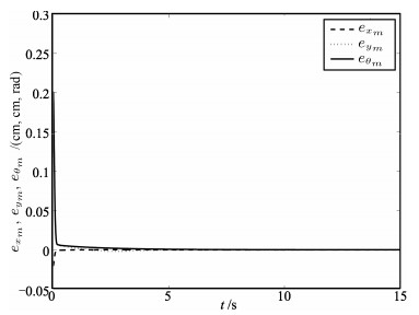
Fig. 9 The tracking error trajectories for ${{e}_{{{x}_{m}}}},{{e}_{{{y}_{m}}}}$ and $e_{\theta_{m}}$ in the image frame for Case 1

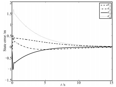
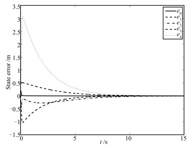
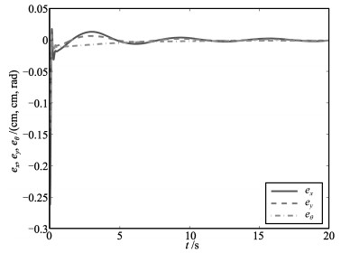
Fig. 10 The tracking error trajectories for ${{e}_{x}},{{e}_{y}}$ and $e_{\theta}$ in the robot task-space for Case 1
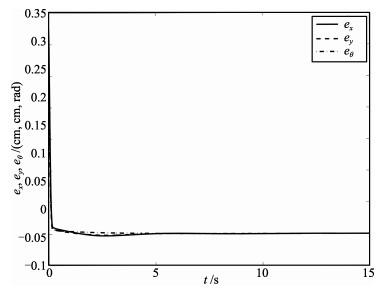
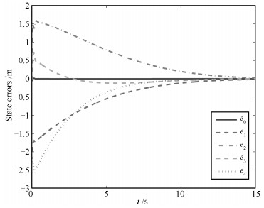
Fig. 13 The tracking error trajectories for ${{e}_{x}},{{e}_{y}}$ and $e_{\theta}$ in the robot task-space for Case 2
-
[1] Kolmanovsky I, McClamroch N H. Developments in nonholonomic control problems. IEEE Control Systems Magazine, 1995, 15(6):20-36 http://cn.bing.com/academic/profile?id=2120944681&encoded=0&v=paper_preview&mkt=zh-cn [2] Wang C L. Semiglobal practical stabilization of nonholonomic wheeled mobile robots with saturated inputs. Automatica, 2008, 44(3):816-822 http://cn.bing.com/academic/profile?id=1967598091&encoded=0&v=paper_preview&mkt=zh-cn [3] Leroquais W, d'Andréa-Novel B. Transformation of the kinematic models of restricted mobility wheeled mobile robots with a single platform into chain forms. In:Proceedings of the 34th Conference on Decision and Control. New Orleans, LA:IEEE, 1995. 3811-3816 [4] Pang Hai-Long, Ma Bao-Li. Adaptive unified controller of arbitrary trajectory tracking for wheeled mobile robots with unknown parameters. Control Theory and Applications, 2014, 31(3):285-292(in Chinese) http://en.cnki.com.cn/Article_en/CJFDTOTAL-KZLY201403003.htm [5] Cao K C. Global κ-exponential tracking control of nonholonomic systems in chained-form by output feedback. Acta Automatica Sinica, 2009, 35(5):568-576 http://cn.bing.com/academic/profile?id=2145479289&encoded=0&v=paper_preview&mkt=zh-cn [6] Ma B L, Tso S K. Unified controller for both trajectory tracking and point regulation of second-order nonholonomic chained systems. Robotics and Autonomous Systems, 2008, 56(4):317-323 http://cn.bing.com/academic/profile?id=2038047332&encoded=0&v=paper_preview&mkt=zh-cn [7] Campion G, Bastin G, Dandrea-Novel B. Structural properties and classification of kinematic and dynamic models of wheeled mobile Robots. IEEE Transactions on Robotics and Automation, 1996, 12(1):47-62 http://cn.bing.com/academic/profile?id=2149012351&encoded=0&v=paper_preview&mkt=zh-cn [8] Jiang Z P. Robust exponential regulation of nonholonomic systems with uncertainties. Automatica, 2000, 36(2):189-209 http://cn.bing.com/academic/profile?id=2079519375&encoded=0&v=paper_preview&mkt=zh-cn [9] Ma Bao-Li. Robust smooth time-varying exponential stabilization of dynamic nonholonomic mobile cart with parameter uncertainties. Acta Automatica Sinica, 2005, 31(2):314-319(in Chinese) http://cn.bing.com/academic/profile?id=2380252068&encoded=0&v=paper_preview&mkt=zh-cn [10] Wang C L, Liang Z Y, Jia Q W. Dynamic feedback robust stabilization of nonholonomic mobile robots based on visual servoing. Journal of Control Theory and Applications, 2010, 8(2):139-144 http://cn.bing.com/academic/profile?id=2084185762&encoded=0&v=paper_preview&mkt=zh-cn [11] Liang Z Y, Wang C L. Robust stabilization of nonholonomic chained form systems with uncertainties. Acta Automatica Sinica, 2011, 37(2):129-142 http://cn.bing.com/academic/profile?id=2081318309&encoded=0&v=paper_preview&mkt=zh-cn [12] Dong W J. On trajectory and force tracking control of constrained mobile manipulators with parameter uncertainty. Automatica, 2002, 38(9):1475-1484 http://cn.bing.com/academic/profile?id=2093817182&encoded=0&v=paper_preview&mkt=zh-cn [13] Wang Y N, Peng J Z, Sun W, Yu H S, Zhang H. Robust adaptive tracking control of robotic systems with uncertainties. Journal of Control Theory and Applications, 2008, 6(3):281-286 http://cn.bing.com/academic/profile?id=1997765899&encoded=0&v=paper_preview&mkt=zh-cn [14] Allen P K, Timcenko A, Yoshimi B, Michelman P. Automated tracking and grasping of a moving object with a robotic hand-eye system. IEEE Transactions on Robotics and Automation, 1993, 9(2):152-165 http://cn.bing.com/academic/profile?id=2109618870&encoded=0&v=paper_preview&mkt=zh-cn [15] Do K D, Jiang Z P, Pan J. Simultaneous tracking and stabilization of mobile robots:an adaptive approach. IEEE Transactions on Automatic Control, 2004, 49(7):1147-1152 http://cn.bing.com/academic/profile?id=2128698518&encoded=0&v=paper_preview&mkt=zh-cn [16] Dixon W E, Dawson D M, Zergeroglu E, Behal A. Adaptive tracking control of a wheeled mobile robot via an uncalibrated camera system. IEEE Transactions on Systems, Man, and Cybernetics——Part B:Cybernetics, 2001, 31(3):341-352 http://cn.bing.com/academic/profile?id=2171694674&encoded=0&v=paper_preview&mkt=zh-cn [17] Jia Bing-Xi, Liu Shan, Zhang Kai-Xiang, Chen Jian. Survey on robot visual servo control:vision system and control strategies. Acta Automatica Sinica, 2015, 41(5):861-873(in Chinese) [18] Chen J, Dixon W E, Dawson M, McIntyre M. Homography-based visual servo tracking control of a wheeled mobile robot. IEEE Transactions on Robotics, 2006, 22(2):406-415 http://cn.bing.com/academic/profile?id=2097671019&encoded=0&v=paper_preview&mkt=zh-cn [19] Wang H S, Liu Y H, Zhou D X. Dynamic visual tracking for manipulators using an uncalibrated fixed camera. IEEE Transactions on Robotics, 2007, 23(3):610-617 http://cn.bing.com/academic/profile?id=2016213375&encoded=0&v=paper_preview&mkt=zh-cn [20] Wang C L, Mei Y C, Liang Z Y, Jia Q W. Dynamic feedback tracking control of non-holonomic mobile robots with unknown camera parameters. Transactions of the Institute of Measurement and Control, 2010, 32(2):155-169 http://cn.bing.com/academic/profile?id=2083474219&encoded=0&v=paper_preview&mkt=zh-cn [21] Yang F, Wang C L. Adaptive tracking control for dynamic nonholonomic mobile robots with uncalibrated camera parameters. In:Proceedings of the 8th Asian Control Conference. Kaohsiung, China:IEEE, 2011. 269-274 http://cn.bing.com/academic/profile?id=2141389837&encoded=0&v=paper_preview&mkt=zh-cn [22] Liang Z Y, Wang C L. Robust exponential stabilization of nonholonomic wheeled mobile robots with unknown visual parameters. Journal of Control Theory and Applications, 2011, 9(2):295-301 http://cn.bing.com/academic/profile?id=2061563135&encoded=0&v=paper_preview&mkt=zh-cn [23] Samson C. Control of chained systems application to path following and time-varying point-stabilization of mobile robots. IEEE Transactions on Automatic Control, 1995, 40(1):64-77 http://cn.bing.com/academic/profile?id=2127988032&encoded=0&v=paper_preview&mkt=zh-cn 期刊类型引用(3)
1. 杨雪梅,陈霞,宋小贝. 基于需求导向理念的康复护理干预对老年脑卒中后吞咽障碍患者吞咽功能及生存质量的影响. 中国当代医药. 2021(04): 231-234 .  百度学术
百度学术2. 陈杰,程胜,徐梦,史豪斌. 面向医疗辅助诊断的可视化多属性决策方法. 计算机工程与应用. 2020(08): 249-255 . 百度学术3. 马宁. 球囊扩张训练式护理对脑出血术后吞咽功能障碍患者吞咽功能的影响. 中国药物与临床. 2020(21): 3683-3685 . 百度学术其他类型引用(1)
-

 下载:
下载:

图(16)
计量
- 文章访问数: 1581
- HTML全文浏览量: 140
- PDF下载量: 791
- 被引次数: 4
