Novel Path Curvature Optimization Algorithm for Intelligent Wheelchair to Smoothly Pass a Narrow Space
-
摘要: 为了使用户更感舒适,智能轮椅应该能在具有复杂几何约束的室内环境下平滑地通过狭窄通道.本文提出一个基于路径曲率优化的算法以确保智能轮椅平滑地通过狭窄过道.考虑到路径平滑度取决于路径曲率及其变化率,在通过传感器数据计算出狭窄通道相对于轮椅的位置后,算法以贝塞尔曲线的曲率及其变化率最小为优化目标,以轮椅过通道时的方向及贝塞尔多边形应为凸多边形作为约束,规划出一条平滑的最优路径,然后控制轮椅实时跟踪这条路径.上述过程动态循环运行,实现了智能轮椅平滑通过狭窄通道.仿真中将本文算法同基于A*的路径规划导航算法进行了对比,结果表明本文提出的基于曲率优化的算法可以实现比A*算法路径曲率更小且更加平滑的过狭窄通道过程,并且即使在没有全局地图和定位信息情况下,算法也能控制轮椅平滑地通过狭窄过道.实验中详细阐述了算法的实现过程,实验结果也证实了算法的有效性.Abstract: This paper presents a novel algorithm to address the smooth narrow pass traversing issue, which is based on optimizing the curvature of the wheelchair path. Being aware of the fact that the path smoothness is determined by the path curvature and its change rate, after calculating the position of the narrow pass relative to the base frame of the wheelchair from perception sensor data, the algorithm takes the curvature and its change rate of Bezier curve as the optimal objective, and the wheelchair heading and the condition that the Bezier curve polygon should be convex polygon as constraints, and plans a smooth and optimal path for the controlled wheelchair to follow. This process is iterated dynamically to enable the intelligent wheelchair to traverse the narrow pass smoothly. Simulation is firstly conducted to compare the performances of our method and the A*-based path planning navigation algorithm, which shows that the proposed algorithm is able to achieve more smooth path with smaller curvature when the wheelchair traverses narrow path. Furthermore, the algorithm can control the wheelchair to traverse narrow pass smoothly even without any global map and localization. Real experiment with detailed explanation of algorithm implementation is also given to verify the effectiveness of the proposed algorithm.
-
Key words:
- Intelligent wheelchair /
- curvature optimization /
- Bezier curve /
- pass traversing
-
1. Introduction
Fractional calculus and fractional differential equations have received considerable interest in the recent forty years. Fractional derivative means that the order of differentiation can be an arbitrary real number and even it can be a complex number. Fractional derivative modelling has been applied to many scientific and engineering fields, such as quantum mechanics [1], viscoelasticity and rheology [2], electrical engineering [3], electrochemistry [4], biology [5], biophysics and bioengineering [6], signal and image processing [7], mechatronics [8], and control theory [9]-[11]. Although few mathematical issues of fractional derivative remain unsolved, most of the difficulties have been overcome, and the applications of fractional calculus in above fields indicate that the fractional models can depict the property and behavior of a real-world problem more accurately. For a comprehensive review of fractional calculus, we refer readers to some monographs [12]-[14] and references therein. In contrast to integer order derivative, the way of identifying fractional derivative is not unique. There are several types of definitions, such as Riemann-Liouville derivative, Caputo derivative, Grünwald-Letnikov derivative, and so on. More details can be found in [13, Chapter 2]. In the recent years, the study of dynamical system with fractional order derivative becomes more and more popular [15]-[19]. Moreover, the dynamics in fractional dynamical system is more interesting.
Returning back to the fractional derivative, since it has several different definitions, how to develop a generalized form which can unify all the existing fractional derivatives becomes one important topic in fractional calculus [20]-[22]. Recently, a class of new generalized fractional integral and generalized fractional derivative is introduced in [22]. The new generalized fractional integral and generalized fractional derivative depend on a scale function and a weight function, which makes them more general. When the scale function and the weight function reduce to some specific cases, the generalized fractional operators will reduce to Riemann-Liouville fractional integral, Riemann-Liouville fractional derivative and Caputo fractional derivative and so on. However, the study of this new generalized fractional integral and generalized fractional derivative are in the very beginning stage now [23]-[26]. In [24], we show that in generalized fractional diffusion equation, the scale function allows the response domain to be scaled differently. It is required that the scale function should be strictly monotonically increasing or decreasing. A convex increasing scale function will compress the response domain towards to the initial time. A concave increasing scale function will stretch the response domain away from the initial time. The weight function allows the response to be assessed differently at different time, since in many applications, we may require an event to be weighed differently at different time point. For example, modeling of memory of a child may require a heavy weight at current time point, whereas the same for an older person may require more weight on the past. To be an initial attempt of application to chaotic dynamical systems, in this paper, we define a class of new generalized fractional chaotic systems by replacing the original derivatives with the new generalized fractional derivative, then apply a finite difference scheme to study the numerical solutions of two different generalized fractional chaotic systems, namely generalized fractional Lotka-Volterra system (GFLVS) and generalized fractional Lorenz system (GFLS). Their complex dynamics will be discussed, and the dynamic behavior depending on the weight and scale function will be shown graphically.
The rest of this paper is organized as follows: In Section 2, the preliminaries of fractional calculus are given. The new generalized fractional integral and generalized fractional derivative are shown. A finite difference approach for solving equations with generalized fractional derivative is carried out. In Section 3, we define the chaotic systems using the generalized fractional derivative of Caputo type, i.e., the GFLVS and GFLS. Some interesting dynamics of those two systems are shown graphically. Finally, the conclusions are drawn in Section 4.
2. Mathematical Preliminaries
In this section, we introduce the preliminaries of generalized fractional derivatives, and show a proper numerical method for differential equations with such derivatives.
2.1 Generalized Fractional Calculus
Let us begin with the common fractional operators. In calculus, the $n$ -fold integral of an integrable function $u(t)$ is defined as
$ I^{n}u(t)=\overbrace{\int^t_0\cdots\int^t_0}^{n\ {\rm times}}u(s)ds\cdots{ds}= \int^t_0\frac{(t-s)^{n-1}}{(n-1)!}u(s)ds $
where $t\geq{0}$ , and $u(0)$ is well-defined. Replacing the positive integer $n$ by a real number $\alpha>0$ , we have the following definition.
Definition 1[13]: The left Riemann-Liouville fractional integral of order $\alpha>0$ of a function $u(t)$ is defined as
$ \begin{align} \left(I^{\alpha}_{0+}u\right)(t) = \frac{1}{\Gamma(\alpha)}\int^t_0(t-s)^{\alpha-1}u(s)ds \end{align} $
(1) provided the integral is finite, where $\Gamma(\alpha)$ is the Gamma function.
The Riemann-Liouville fractional integral plays an important role in defining fractional derivatives. There are two basic approaches to define the fractional derivative, i.e., "first integration then differentiation" and "first differentiation then integration". The corresponding fractional derivatives are called Riemann-Liouville fractional derivative and Caputo fractional derivative, and the definitions are given as follows.
Definition 2[13]:The left Riemann-Liouville fractional derivative of order $n-1 < \alpha < n$ of a function $u(t)$ is defined as
$ \begin{align} \left(D^{\alpha}_{0+}u\right)(t) = \frac{1}{\Gamma(n-\alpha)}\left(\frac{d^n}{dt^n}\right) \int^t_0(t-s)^{n-\alpha-1}u(s)ds \end{align} $
(2) provided the right side of the identity is finite.
Definition 3[13]: The left Caputo fractional derivative of order $n-1 < \alpha < n$ of a function $u(t)$ is defined as
$ \begin{align} \left({^cD}^{\alpha}_{0+}u\right)(t) = \frac{1}{\Gamma(n-\alpha)}\int^t_0(t-s)^{n-\alpha-1}u^{(n)}(s)ds \end{align} $
(3) provided the right side of the identity is finite.
Besides above, there also exist right Riemann-Liouville integral and derivative, and right Caputo fractional derivative [13]. Mathematically, the Riemann-Liouville and Caputo fractional operators are used in applications frequently. In most real-world models, we always employ the left Caputo fractional derivative. One reason is that we will study generalized fractional dynamical system later, and the derivative is taken with respect to time variable. In physical models, time is always running forward. The other reason is that in the differential equations with Caputo fractional derivative, the initial conditions are taken in the same form as for integer-order differential equations which have clear physical meanings in the practical application and can be easily measured [14]. In what follows, we will introduce the generalized fractional integral and derivative proposed in [22]. They extend nearly all the existing fractional operators. Now we list the generalized fractional integral and derivative defined on positive half axis. They will be used to define the generalized fractional chaotic systems in next section.
Definition 4[22]: The left generalized fractional integral of order $\alpha>0$ of a function $u(t)$ with respect to a scale function $\sigma(t)$ and a weight function $w(t)$ is defined as
$ \begin{align} \left(I^{\alpha}_{0+;[\sigma, w]}u\right)(t) = \frac{[w(t)]^{-1}}{\Gamma(\alpha)}\int^{t}_{0} \frac{w(s)\sigma'(s)u(s)}{[\sigma(t)-\sigma(s)]^{1-\alpha}}ds \end{align} $
(4) provided the integral exists, where $\sigma'(s)$ indicates the first derivative of the scale function $\sigma$ .
Definition 5[22]: The left generalized derivative of order $m$ of a function $u(t)$ with respect to a scale function $\sigma(t)$ and a weight function $w(t)$ is defined as
$ \begin{align} \left(D^m_{[\sigma, w;L]}u\right)(t) = [w(t)]^{-1}\left[\left(\frac{1}{\sigma'(t)}D_t\right)^m(w(t)u(t))\right] \end{align} $
(5) provided the right-side of equation is finite, where $m$ is a positive integer.
Definition 6[22]: The Caputo type left generalized fractional derivative of order $\alpha>0$ of a function $u(t)$ with respect to a scale function $\sigma(t)$ and a weight function $w(t)$ is defined as
$ \begin{align} \left(D^{\alpha}_{0+;[\sigma, w]}u\right)(t) = \left(I^{m-\alpha}_{0+;[\sigma, w]}D^m_{[\sigma, w;L]}u\right)(t) \end{align} $
(6) provided the right-side of equation is finite, where $m-1\leq$ $\alpha$ $ < $ $m$ , and $m$ is a positive integer. Particularly, when $0 < $ $\alpha$ $ < $ $1$ , we have
$ \begin{align} \left(D^{\alpha}_{0+;[\sigma, w]}u\right)(t) = \frac{[w(t)]^{-1}}{\Gamma(1-\alpha)}\int^{t}_{0} \frac{[w(s)u(s)]'}{[\sigma(t)-\sigma(s)]^{\alpha}}ds. \end{align} $
(7) 2.2 Finite Difference Method
Now we introduce a finite difference method for solving differential equations with generalized fractional derivative. Consider the following generalized fractional differential equation:
$ \begin{align} \begin{cases} \left(D^{\alpha}_{0+;[\sigma, w]}u\right)(t)=f(t, u(t)), \quad 0 < t\leq T\\ u(0)=u_0 \end{cases} \end{align} $
(8) where $0 < \alpha < 1$ and $T$ is the final time. Without loss of generality, on a uniform mesh $0=t_0 < t_1 < \cdots < $ $t_j < $ $t_{j+1} < \cdots < t_N=T$ , the Caputo type generalized fractional derivative of $u(t)$ can be approximated as
$ \begin{align} (D^{\alpha}_{0+;[\sigma, w]}& u)(t_{j+1}) \nonumber\\ &= \frac{[w(t_{j+1})]^{-1}}{\Gamma(1-\alpha)}\int^{t_{j+1}}_{0}\frac{[w(s)u(s)]'} {[\sigma(t_{{j+1}})-\sigma(s)]^{\alpha}}ds \nonumber\\ &= \frac{w_{j+1}^{-1}}{\Gamma(1-\alpha)}\sum^{j}_{k=0}\int^{t_{k+1}}_{t_k} \frac{[w(s)u(s)]'}{\left[\sigma(t_{{j+1}})-\sigma(s) \right]^{\alpha}}ds \nonumber\\ & \approx \frac{w_{j+1}^{-1}}{\Gamma(1-\alpha)}\sum^{j}_{k=0}\int^{t_{k+1}}_{t_k} \frac{\frac{w_{k+1}u_{k+1}-w_ku_k}{t_{k+1}-t_k}} {\left[\sigma_{j+1}-\sigma(s)\right]^{\alpha}}ds \nonumber\\ & \approx\sum^{j}_{k=0}\left(A^j_ku_{k+1}-B^j_ku_k\right) \end{align} $
(9) where
$ \begin{align*} A^j_k =&\ \frac{w^{-1}_{j+1}w_{k+1}}{\Gamma(2-\alpha)(\sigma_{k+1}-\sigma_k)} \\ & \times \left[(\sigma_{j+1}-\sigma_k)^{1-\alpha}- (\sigma_{j+1}-\sigma_{k+1})^{1-\alpha}\right]\\ B^j_k =&\ \frac{w^{-1}_{j+1}w_{k}}{\Gamma(2-\alpha)(\sigma_{k+1}-\sigma_k)} \\ & \times \left[(\sigma_{j+1}-\sigma_k)^{1-\alpha}- (\sigma_{j+1}-\sigma_{k+1})^{1-\alpha}\right] \end{align*} $
$k=0, 1, 2, \ldots, j$ , $u_j=u(t_j)$ , $w_j=w(t_j)$ , and $\sigma_j=\sigma(t_j)$ .
Therefore, we obtain the finite difference scheme:
$ \begin{align} \sum^{j}_{k=0}\left(A^j_ku_{k+1}-B^j_ku_k\right)=f(t_{j+1}, u_{j+1}) \end{align} $
(10) and the corresponding iteration scheme as
$ \begin{align} u_{j+1}=\begin{cases} \frac{1}{A^j_j}\left[f_j-\sum\limits^{j-1}_{k=0} \left(A^j_ku_{k+1}-B^j_ku_k\right)+B^j_ju_j \right], \\ \qquad \qquad \qquad \qquad \qquad\qquad j=1, 2, \ldots, N-1\\ \frac{1}{A^0_0}\left(f_0+B^0_0u_0\right), \qquad\qquad \ \, j=0 \end{cases} \end{align} $
(11) where $f_j=f(t_j, u_j)$ .
In what follows, we will apply this method to solve the generalized fractional chaotic systems. The numerical analysis of the above scheme can be found in [26].
3. Dynamic Behavior of Generalized Fractional Chaotic Systems
In this section, we introduce two nonlinear dynamical systems but redefine them with Caputo type generalized fractional derivative. The classical and fractional senses are special cases of the new generalized fractional system below.
3.1 Generalized Fractional Lotka-Volterra and Generalized Fractional Lorenz System
Replacing the derivative with the generalized fractional derivative defined by (7), we define the generalized fractional Lotka-Volterra system (GFLVS) as
$ \begin{align} \begin{cases} D^{\alpha_1}_{0+;[\sigma, w]}x = ax - bxy + mx^2 - sx^2z\\ D^{\alpha_2}_{0+;[\sigma, w]}y = -cy +dxy\\ D^{\alpha_3}_{0+;[\sigma, w]}z = -pz + sx^2z \end{cases} \end{align} $
(12) where $0 < \alpha_1, \alpha_2, \alpha_3 < 1$ ( $\alpha_1$ , $\alpha_2$ , $\alpha_3$ can be the equal or different) are the orders of the derivative and parameters $a$ , $b$ , $c$ , $d$ are positive. $a$ represents the natural growth rate of the prey in the absence of predators, $b$ represents the effect of predator on the prey, $c$ represents the natural death rate of the predator in the absence of prey, $d$ represents the efficiency and propagation rate of the predator in the presence of prey, and $m$ , $p$ , $s$ are positive constants.
By selecting the parameters $a=1$ , $b=1$ , $c=1$ , $d=1$ , $m$ $=$ $2$ , $s=2.7$ , $p=3$ and the initial condition $[x_0, y_0, z_0]$ $=$ $[1.5, 1.5, 1.5]$ , when $\alpha_1=\alpha_2=\alpha_3=0.95$ , (12) represents the generalized fractional Lotka-Volterra chaotic system and the phase portraits of the system (12) are described through Figs. 1(a) and 1(b). In Fig. 1(a), the chaotic phenomenon is shown. Moreover, the GFLVS reduces to the fractional Lotka-Volterra system as $\sigma(t)=t$ and $w(t)=1$ . In Fig. 1(b), we see that when the scale function is specified as a power function, and the weight function is taken as an exponential function, the chaotic attractor vanishes and then a stable equilibrium point appears.
Similarly, we define the generalized fractional Lorenz system (GFLS) as
$ \begin{align} \begin{cases} D^{\alpha_1}_{0+;[\sigma, w]}x = r(y-x)\\ D^{\alpha_2}_{0+;[\sigma, w]}y = x(\rho-z)-y\\ D^{\alpha_3}_{0+;[\sigma, w]}z = xy-\beta{z} \end{cases} \end{align} $
(13) where $r$ is the Prandtl number, $\rho$ is the Rayleigh number and $\beta$ is the size of the region approximated by the system. The fractional order $0 < \alpha_1, \alpha_2, \alpha_3 < 1$ may take different values.
By taking the parameters $r=10$ , $\rho=28$ , $\beta= {8}/{3}$ , and the initial condition $[x_0, y_0, z_0]=[0.5, 0.5, 0.5]$ , when $\alpha_1$ $=$ $\alpha_2=\alpha_3=0.99$ , (13) represents the generalized fractional Lorenz chaotic system and the phase portraits of the system (13) are described through Figs. 1(c) and 1(d). In Fig. 1(c), the chaotic attractor of fractional Lorenz system is presented. When we take scale function as a power function, and weight function as exponential function, the GFLS remains chaotic. However, the shape of the attractor changes, which is shown in Fig. 1(d).
3.2 Analysis of the Influence of Scale and Weight Functions
Now we analyze the influence of the scale and weight functions on the responses of generalized fractional differential equation. For simplicity, we consider
$ \begin{align} D^{\alpha}_{0+;[\sigma, w]}u(t) = Au(t) + f(t) \end{align} $
(14) where $A\neq{0}$ is a constant.
Equation (14) is equivalent to
$ \begin{align} \frac{[w(t)]^{-1}}{\Gamma(1-\alpha)}\int^{t}_{0} \frac{[w(s)u(s)]'}{[\sigma(t)-\sigma(s)]^{\alpha}}ds = Au(t) + f(t). \end{align} $
(15) Let $v(t) = w(t)u(t)$ , we have
$ \begin{align} \frac{1}{\Gamma(1-\alpha)}\int^{t}_{0} \frac{v(s)'}{[\sigma(t)-\sigma(s)]^{\alpha}}ds = Av(t) + w(t)f(t). \end{align} $
(16) According to [13], we deduce the solution of (16) as:
$ \begin{align} v(t) =&\ E_{\alpha}\left(A[\sigma(t)-\sigma(0)]^{\alpha}\right)v_0 \nonumber\\ & +\int^t_0(\sigma(t)-\sigma(s))^{\alpha-1} \nonumber\\ &\times E_{\alpha, \alpha}[A(\sigma(t)-\sigma(s))^{\alpha}]w(s)f(s)ds \end{align} $
(17) which implies that
$ \begin{align} u(t)=&\ \frac{w(0)}{w(t)}E_{\alpha}\left(A[\sigma(t)-\sigma(0)]^{\alpha}\right)u_0 \nonumber\\ & +\frac{1}{w(t)}\int^t_0(\sigma(t)-\sigma(s))^{\alpha-1} \nonumber\\ & \times E_{\alpha, \alpha}[A(\sigma(t)-\sigma(s))^{\alpha}]w(s)f(s)ds \end{align} $
(18) where $u_0$ is the initial condition, and $E$ is the Mittag-Leffler function.
In (18), we observe that how the weight and scale functions influence the behavior of (14). First of all, the weight function cannot be zero in the domain, otherwise solution $u(t)$ will go to infinity. Second, the scale function cannot be periodic, and if it is, the generalized fractional derivative will be infinity at $t=s$ . For an intuitive comprehension, we present some numerical simulations in the following.
3.3 Dynamics of GFLVS and GFLS Depend on Scale and Weight Functions
The fractional chaotic systems are sufficiently generalized by using the generalized fractional derivative, since many existing fractional derivatives, as well as integer order derivatives, are special cases of the generalized fractional derivative. In our numerical experiments, we find many interesting dynamical behaviors of generalized fractional chaotic systems which are never found in common fractional or integer order chaotic systems. Here we present some particular simulation results. However, our discussion depends on Figs. 2 and 3, and others figures are not shown here.
First, we simulate the influence of scale function on dynamics of chaotic systems. In GFLVS, we take fractional order $\alpha_1=\alpha_2=\alpha_3=0.95$ , weight function $w(t)=\exp(1.2t)$ , and other parameters are the same as before. In GFLS, we select fractional order $\alpha_1=\alpha_2=\alpha_3=0.99$ , weight function $w(t)=\exp(0.1t)$ , and other parameters are the same as before. The dynamic behaviors of GFLVS and GFLS with scale function $\sigma(t)=t$ and $t^{1.14}$ are individually presented in Fig. 2.
Second, we simulate the influence of weight function on dynamics of chaotic systems. In GFLVS, we take fractional order $\alpha_1=\alpha_2=\alpha_3=0.95$ , scale function $\sigma(t)=t$ , and other parameters are the same as before. In GFLS, we select fractional order $\alpha_1=\alpha_2=\alpha_3=0.99$ , scale function $\sigma(t)=t$ , and other parameters are the same as before. The dynamic behaviors of GFLVS with weight function $w(t)$ $=$ $\exp(0.8t)$ , $\exp(1.3t)$ , and GFLS with weight function $w(t)=\exp(2+0.5t)$ and $\exp(2+0.2t)$ are presented in Fig. 3.
Finally, to end this section, we make some remarks based on the numerical experiments above. Some other figures are not listed here for shortening the length of paper.
1) The GFLVS is chaotic with scale function $\sigma(t)=t$ , weight function $w(t)$ is a nonzero constant, and fractional order $\alpha_i=0.95$ , $i=1, 2, 3$ [27]. However, From Fig. 1(a), Fig. 2(a) and Fig. 3(a), we may see that as the weight function varies, the chaotic attractor vanishes and then a limit cycle emerges or the system converges to a stable equilibrium point. Furthermore, from Fig. 2(a) and Fig. 2(b), we observe that as the scale function varies, the limit cycle tends to be a stable equilibrium point. From Fig. 3(a) and Fig. 3(b), it is shown that as the weight function varies, the limit cycle can be generated from a stable equilibrium point.
2) The GFLS is chaotic with scale function $\sigma(t)=t$ , weight function $w(t)$ is a nonzero constant, and fractional order $\sum^{3}_{i=1}\alpha_i>2.91$ [28]. In simulation, on one hand, Figs. 1(c) and 1(d), indicate that with suitable scale and weight functions, the GFLS also has a chaotic attractor. On the other hand, Fig. 1(c), Fig. 1(d), Fig. 2(c), Fig. 2(d), and Fig. 3(d) imply that the scale and weight functions can influence the shape and position of chaotic attractor. From Figs. 3(c) and 3(d), we observe that with some suitable weight function, the chaotic attractor tends to be an asymptotically stable equilibrium point.
3) Our previous work [23]-[26] verified that in generalized fractional integral and generalized fractional derivative, the basic property of scale function $\sigma(t)$ is that it changes the time axis, which means that if the time domain is specified as $[0, T]$ , then the response of the dynamical system is obtained over $[\sigma(0), \sigma(T)]$ , provided the scale function is monotone increasing. Since the chaotic dynamical systems are sensitive to the initial conditions, when we take different scale functions in generalized fractional chaotic system, many different dynamical behaviors will be drawn.
4) A similar observation to weight function can be found in [23]-[26], which shows that in generalized fractional integral and generalized fractional derivative, the basic property of weight function $w(t)$ is that it puts different weights for function in different positions of domain. The classical fractional operators have memory property which makes them excellent tools to model the diffusion process with heredity. Generally, in left Caputo type generalized fractional derivative, the monotonic increasing weight function is coincident with the inner memory property of fractional operator, while the monotonic decreasing weight function can destroy this inner property. One can also follow our numerical method and try other scale and weight functions in numerical experiments.
5) In Figs. 2 and 3, one can observe that both changing the scale and weight functions make the systems change between different dynamical behavior (e.g., limit cycle and stable equilibrium point). These phenomena can be regarded as general cases for generalized fractional chaotic systems. We shall guess that either scale function or weight function would influence the dynamics of generalized fractional chaotic systems. In Fig. 2, the weight function is fixed so that the influence of scale function on GFLVS and GFLS is presented. Similarly, in Fig. 3, the scale function is fixed so that the influence of weight function on GFLVS and GFLS is shown. From (18), we clearly see that the scale function plays an important role in scaling the long time behavior of dynamics since it is located in the generalized exponential function, and the weight function provides a different average since it lies inside the integral, and it is a variable coefficient simultaneously. Apparently, the behavior of function $u$ depends on the changing of scale and weight functions.
4. Conclusions
In this paper, we presented a class of new generalized fractional chaotic system, using the new generalized fractional derivative proposed recently. Many dynamical systems with integer or fractional order derivatives can be extended by replacing the derivative with the generalized fractional derivative. Therefore, the new generalized fractional dynamical systems considered in this paper can exhibit more complex dynamic behaviors. In simulations, we show that the dynamical behaviors of such systems not only depend on fractional order, but also depend on the scale and weight functions.
Acknowledgement: The author is grateful to Professor O. P. Agrawal (SIUC, USA) for introducing him theory of generalized fractional calculus, suggesting the basic idea of this paper, as well as his kind help and continuous encouragement in the recent years.
-
表 1 每条路径的输入参数
Table 1 The input parameters for each path
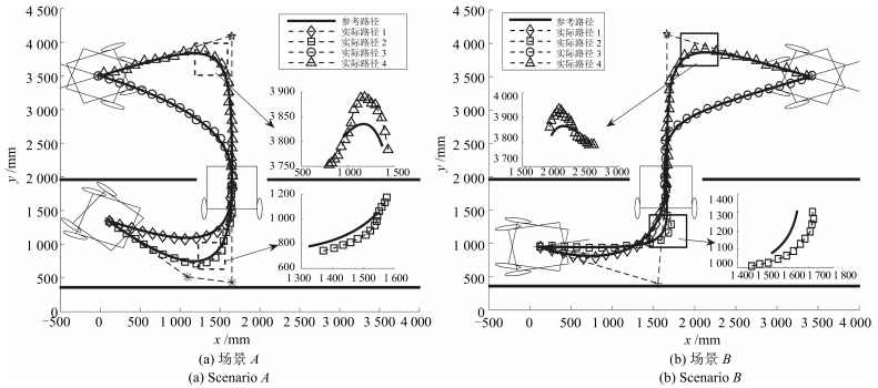
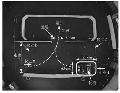
场景 Ps (m) Pd (m) Pt (m) 1 (Hs, Hd) 2 (Hs, Hd) 3 (Hd, Ht) 4 (Hd, Ht) A (0.1, 1.3) (1.6, 1.8) (0.0, 3.5) (-20, 90) (-40, 90) (90, 160) (90, 200) B (0.1, 1.3) (1.6, 1.8) (3.4, 3.5) (-10, 90) (10, 90) (90, 20) (90, -20) -
[1] Elbanhawi M, Simic M, Jazar R N. Continuous path smoothing for car-like robots using B-spline curves. Journal of Intelligent and Robotic Systems, 2015, 80(1):23-56 http://www.academia.edu/15534117/Continuous_Path_Smoothing_for_Car-Like_Robots_Using_B-Spline_Curves [2] Yoon S, Yoon S E, Lee U, Shim D H. Recursive path planning using reduced states for car-like vehicles on grid maps. IEEE Transactions on Intelligent Transportation Systems, 2015, 16(5):2797-2813 doi: 10.1109/TITS.2015.2422991 [3] Pan Z, Li J Q, Hu K M, Zhu H. Intelligent vehicle path planning based on improved artificial potential field method. Applied Mechanics and Materials, 2014, 742:349-354 https://www.researchgate.net/publication/276868213_Intelligent_Vehicle_Path_Planning_Based_on_Improved_Artificial_Potential_Field_Method [4] 张浩杰, 龚建伟, 姜岩, 熊光明, 陈慧岩.基于变维度状态空间的增量启发式路径规划方法研究.自动化学报, 2013, 39(10):1602-1610 doi: 10.3724/SP.J.1004.2013.01602Zhang Hao-Jie, Gong Jian-Wei, Jiang Yan, Xiong Guang-Ming, Chen Hui-Yan. Research on incremental heuristic path planner with variable dimensional state space. Acta Automatica Sinica, 2013, 39(10):1602-1610 doi: 10.3724/SP.J.1004.2013.01602 [5] 祖迪, 韩建达, 谈大龙.加速度空间中基于线性规划的移动机器人路径规划方法.自动化学报, 2007, 33(10):1036-1042 http://www.aas.net.cn/CN/abstract/abstract13407.shtmlZu Di, Han Jian-Da, Tan Da-Long. LP-based path planning method in acceleration space for mobile robot. Acta Automatica Sinica, 2007, 33(10):1036-1042 http://www.aas.net.cn/CN/abstract/abstract13407.shtml [6] Park J W, Im W S, Kim D Y, Kim J M. Safe driving algorithm of the electric wheelchair with model following control. In:Proceedings of the 16th European Conference on Power Electronics and Applications. Lappeenranta, Finland:IEEE, 2014. 1-10 [7] Sinyukov D A, Padir T. Adaptive motion control for a differentially driven semi-autonomous wheelchair platform. In:Proceedings of the 2015 International Conference on Advanced Robotics. Istanbul, Turkey:IEEE, 2015. 288-294 [8] Zhang Z Y, Zhao Z P. A multiple mobile robots path planning algorithm based on a-star and Dijkstra algorithm. International Journal of Smart Home, 2014, 8(3):75-86 doi: 10.14257/ijsh [9] Bhadoria A, Singh R K. Optimized angular a star algorithm for global path search based on neighbor node evaluation. International Journal of Intelligent Systems and Applications, 2014, 6(8):46-52 doi: 10.5815/ijisa [10] Seder M, Mostarac P, Petrović I. Hierarchical path planning of mobile robots in complex indoor environments. Transactions of the Institute of Measurement and Control, 2011, 33(3-4):332-358 doi: 10.1177/0142331208100107 [11] BSI. Design of Buildings and Their Approaches to Meet the Needs of Disabled People. Code of Practice. Standard Number BS 8300:2009+A1:2010, ISBN 9780580707308, British Standards Institute, 2009. [12] Cheein F, De La Cruz C, Guimaraes E, Bastos-Filho T, Carelli R. Navigation system for UFES's robotic wheelchair. Devices for Mobility and Manipulation for People with Reduced Abilities. Boca Raton, FL:CRC Press, 2014. 41-93 [13] Peula J M, Urdiales C, Herrero I, Fernandez-Carmona M, Sandoval F. Case-based reasoning emulation of persons for wheelchair navigation. Artificial Intelligence in Medicine, 2012, 56(2):109-121 doi: 10.1016/j.artmed.2012.08.007 [14] Rastelli J R, Lattarulo R, Nashashibi F. Dynamic trajectory generation using continuous-curvature algorithms for door to door assistance vehicles. In:Proceedings of the 2014 IEEE Intelligent Vehicles Symposium. Dearborn, USA:IEEE, 2014. 510-515 [15] Brezak M, Petrović I. Real-time approximation of clothoids with bounded error for path planning applications. IEEE Transactions on Robotics, 2014, 30(2):507-515 doi: 10.1109/TRO.2013.2283928 [16] Chu C H, Hsieh H T, Lee C H, Yan C Y. Spline-constrained tool-path planning in five-axis flank machining of ruled surfaces. The International Journal of Advanced Manufacturing Technology, 2015, 80(9-12):2097-2104 doi: 10.1007/s00170-015-7201-4 [17] Simba K R, Uchiyama N, Sano S. Real-time smooth trajectory generation for nonholonomic mobile robots using Bézier curves. Robotics and Computer-Integrated Manufacturing, 2016, 41(1):31-42 https://www.researchgate.net/publication/297587735_Real-time_smooth_trajectory_generation_for_nonholonomic_mobile_robots_using_Bezier_curves [18] Yang L, Song D L, Xiao J Z, Han J D, Yang L Y, Cao Y. Generation of dynamically feasible and collision free trajectory by applying six-order Bezier curve and local optimal reshaping. In:Proceedings of the 2015 IEEE/RSJ International Conference on Intelligent Robots and Systems (IROS). Hamburg, Germany:IEEE, 2015. 643-648 [19] Wu J, Snášel V. A Bézier curve-based approach for path planning in robot soccer. In:Proceedings of the 4th International Conference on Innovations in Bio-inspired Computing and Applications. Ostrava, Czech Republic:Springer International Publishing, 2014. 105-113 [20] 陈成, 何玉庆, 卜春光, 韩建达.基于四阶贝塞尔曲线的无人车可行轨迹规划.自动化学报, 2015, 41(3):486-496 http://www.aas.net.cn/CN/abstract/abstract18627.shtmlChen Cheng, He Yu-Qing, Bu Chun-Guang, Han Jian-Da. Feasible trajectory generation for autonomous vehicles based on quartic Bézier curve. Acta Automatica Sinica, 2015, 41(3):486-496 http://www.aas.net.cn/CN/abstract/abstract18627.shtml [21] Choi J W, Curry R, Elkaim G. Piecewise Bezier curves path planning with continuous curvature constraint for autonomous driving. Machine Learning and Systems Engineering. Netherlands:Springer, 2010. 31-45 [22] Hart P E, Nilsson N J, Raphael B. A formal basis for the heuristic determination of minimum cost paths. IEEE Transactions on Systems Science and Cybernetics, 1968, 4(2):100-107 doi: 10.1109/TSSC.1968.300136 [23] Open Source Robotics Foundation (OSRF). Robot operating system[Online], available:http://www.ros.org, May 21, 2016 [24] Open Source Robotics Foundation (OSRF). Gazebo[Online], available:http://www.gazebosim.org/, May 21, 2016 [25] Open Source Robotics Foundation (OSRF). Global planner of navigation stack in ROS[Online], available:http://wiki.ros.org/global_planner?distro=indigo, May 21, 2016 [26] Borges G A, Aldon M J. Line extraction in 2D range images for mobile robotics. Journal of Intelligent and Robotic Systems, 2004, 40(3):267-297 doi: 10.1023/B:JINT.0000038945.55712.65 [27] Duda R O, Hart P E. Pattern Classification and Scene Analysis. New York:Wiley, 1973. 期刊类型引用(3)
1. 曾超,王文军,陈朝阳,张超飞,成波. 模拟驾驶实验中同步装置设计及实验教学应用. 实验技术与管理. 2020(03): 99-102 . 百度学术
2. 吴思凡,杜煜,徐世杰,杨硕,杜晨. 基于长短期记忆-异步优势动作评判的智能车汇入模型. 汽车技术. 2019(10): 42-47 . 百度学术
3. 成英,高利,陈雪梅,赵亚男. 有人与无人驾驶车辆交叉口驾驶博弈模型. 北京理工大学学报. 2019(09): 938-943 . 百度学术
其他类型引用(17)
-