图像理解中的卷积神经网络

常亮; 邓小明; 周明全; 武仲科; 袁野; 杨硕; 王宏安

doi:10.16383/j.aas.2016.c150800

图像理解中的卷积神经网络

doi: 10.16383/j.aas.2016.c150800

常亮^1,2,,
邓小明^3, ,,
周明全^1,2,,
武仲科^1,2,,
袁野^3,4,,
杨硕^3,4,,
王宏安^3,

1.
北京师范大学信息科学与技术学院北京 100875
2.
教育部虚拟现实应用工程研究中心北京 100875
3.
中国科学院软件研究所人机交互北京市重点实验室北京 100190
4.
中国科学院大学计算机与控制学院北京 100049

基金项目:

国家自然科学基金 61473276

国家自然科学基金 61402040

详细信息

作者简介:
常亮北京师范大学信息科学与技术学院副教授.主要研究方向为计算机视觉与机器学习.E-mail:changliang@bnu.edu.cn

周明全北京师范大学信息科学与技术学院教授.主要研究方向为计算机可视化技术,虚拟现实.E-mail:mqzhou@bnu.edu.cn

武仲科北京师范大学信息科学与技术学院教授.主要研究方向为计算机图形学,计算机辅助几何设计,计算机动画,虚拟现实.E-mail:zwu@bnu.edu.cn

袁野中国科学院软件研究所硕士研究生.主要研究方向为计算机视觉.E-mail:yuanye13@mails.ucas.ac.cn

杨硕中国科学院软件研究所硕士研究生.主要研究方向为计算机视觉.E-mail:yangshuo114@mails.ucas.ac.cn

王宏安中国科学院软件研究所研究员.主要研究方向为实时智能,自然人机交互.E-mail:hongan@iscas.ac.cn

通讯作者:
邓小明中国科学院软件研究所副研究员.主要研究方向为计算机视觉.本文通信作者.E-mail:xiaoming@iscas.ac.cn

计量
- 文章访问数: 8779
- HTML全文浏览量: 3432
- PDF下载量: 7329
- 被引次数: 0
出版历程
- 收稿日期: 2015-12-11
- 录用日期: 2016-05-03
- 刊出日期: 2016-09-01

Convolutional Neural Networks in Image Understanding

CHANG Liang^{1,2
,},
DENG Xiao-Ming^{3
, ,},
ZHOU Ming-Quan^{1,2
,},
WU Zhong-Ke^{1,2
,},
YUAN Ye^{3,4
,},
YANG Shuo^{3,4
,},
WANG Hong-An^3
,

1.
College of Information Science and Technology, Beijing Normal University, Beijing 100875
2.
Engineering Research Center of Virtual Reality and Applications, Ministry of Education, Beijing 100875
3.
Beijing Key Laboratory of Human-Computer Interactions, Institute of Software, Chinese Academy of Sciences, Beijing 100190
4.
School of Computer and Control Engineering, University of Chinese Academy of Sciences, Beijing 100049

Funds:

National Natural Science Foundation of China 61473276

National Natural Science Foundation of China 61402040

More Information

Author Bio:
Associate professor at the College of Information Science and Technology, Beijing Normal University. Her research interest covers computer vision and machine learning.

Professor at the College of Information Science and Technology, Beijing Normal University. His research interest covers information visualization and virtual reality.

Professor at the College of Information Science and Technology, Beijing Normal University. His research interest covers computer graphics, computer-aided design, computer animation, and virtual reality.

Master student at the Institute of Software, Chinese Academy of Sciences. His main research interest is computer vision.

Master student at the Institute of Software, Chinese Academy of Sciences. His main research interest is computer vision.

Professor at the Institute of Software, Chinese Academy of Sciences. His research interest covers real-time intelligence and natural human-computer interactions.

Corresponding author: DENG Xiao-Ming Associate professor at the Institute of Software, Chinese Academy of Sciences. His main research interest is computer vision. Corresponding author of this paper.

摘要

摘要: 近年来，卷积神经网络（Convolutional neural networks，CNN）已在图像理解领域得到了广泛的应用，引起了研究者的关注. 特别是随着大规模图像数据的产生以及计算机硬件（特别是GPU）的飞速发展，卷积神经网络以及其改进方法在图像理解中取得了突破性的成果，引发了研究的热潮. 本文综述了卷积神经网络在图像理解中的研究进展与典型应用. 首先，阐述卷积神经网络的基础理论;然后，阐述其在图像理解的具体方面，如图像分类与物体检测、人脸识别和场景的语义分割等的研究进展与应用.
- 卷积神经网络 /
- 图像理解 /
- 深度学习 /
- 图像分类 /
- 物体检测
Abstract: Convolutional neural networks (CNN) have been widely applied to image understanding, and they have arose much attention from researchers. Specifically, with the emergence of large image sets and the rapid development of GPUs, convolutional neural networks and their improvements have made breakthroughs in image understanding, bringing about wide applications into this area. This paper summarizes the up-to-date research and typical applications for convolutional neural networks in image understanding. We firstly review the theoretical basis, and then we present the recent advances and achievements in major areas of image understanding, such as image classification, object detection, face recognition, semantic image segmentation etc.
- Convolutional neural networks (CNN) /
- image understanding /
- deep learning /
- image classification /
- object detection

HTML全文

图 1 卷积神经网络示例

Fig. 1 Illustration of convolutional neural networks

下载: 全尺寸图片幻灯片

图 2 AlexNet卷积神经网络结构示意图^[8]

Fig. 2 Network architecture of AlexNet convolutional neural networks^[8]

下载: 全尺寸图片幻灯片

图 3 基于卷积神经网络的关节检测方法^[63]

Fig. 3 Hand joint detection with convolutional neural networks^[63]

下载: 全尺寸图片幻灯片

表 1 ImageNet竞赛历年来图像分类任务的部分领先结果

Table 1 Representative top ranked results in image classification task of "ImageNet Large Scale Visual Recognition Challenge"

公布时间	机构	Top-5错误率
2015.12.10	MSRA	3.57^[15]
2014.8.18	Google	6.66^[11]
2014.8.18	Oxford	7.33^[12]
2013.11.14	NYU	11.7
2012.10.13	U.Toronto	16.4^[8]

下载: 导出CSV

表 2 部分具有代表性的图像分类和物体检测模型对比

Table 2 Comparison of representative image classification and object detection models

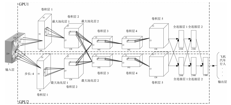
方法	输入	优点	缺点
AlexNet^[8]	整张图像(需要对图像放缩到固定大小)	网络简单易于训练, 对图像分类有较强的鉴别力	网络输入图像要求固定大小, 容易破环物体的纵横比和上下文信息
GoogLeNet^[11]	整张图像(需要对图像放缩到固定大小)	对图像分类拥有非常强的鉴别力, 参数相对AlexNet较少	网络复杂, 对样本数量要求较高, 训练耗时
VGG^[12]	整张图像(需要对图像放缩到固定大小)	对图像分类拥有非常强的鉴别力	网络复杂, 对样本数量要求较高, 训练耗时, 需要多次对网络参数的微调
DPM^[23]	整张图像	对物体检测拥有较强的鉴别力, 对形变和遮挡具有一定的处理能力	使用人工设计的HOG特征^[26]; 对物体检测的精度通常比本表中其他的CNN网络低
R-CNN^[9]	图像区域	对物体检测拥有很强的鉴别力; 比在图像金字塔上逐层滑动窗口的物体检测方法效率高;使用包围盒回归(Bounding box regression)提高物体的定位精度	依赖于区域选择算法; 网络输入图像要求固定大小, 容易破环物体的纵横比和上下文信息; 训练是多阶段过程:在特定检测数据集上对网络参数进行微调、提取特征、训练SVM (Sup-port vector machine)分类器、包围盒回归(Bounding box regression);训练时间耗时、耗存储空间
SPP-net^[10]	整张图像(不要求固定大小)	对物体检测拥有很强的鉴别力, 输入图像可以任意大小, 可保证图像的比例信息训练速度比R-CNN快3倍左右, 测试比R-CNN快10~100倍	网络结构复杂时, 池化对图像造成一定的信息丢失; SPP层前的卷积层不能进行网络参数更新^[24]; 训练是多阶段过程:在特定检测数据集上对网络参数进行微调、提取特征、训练SVM分类器、包围盒回归; 训练时间耗时、耗存储空间
Fast R-CNN^[24]	整张图像(不要求固定大小)	训练和测试都明显快于SPP-net (除了候选区域提取以外的环节接近于实时), 对物体检测拥有很强的鉴别力, 输入图像可以任意大小, 保证图像比例信息, 同时进行分类与定位	依赖于候选区域选择, 它仍是计算瓶颈
Faster R-CNN^[29]	整张图像(不要求固定大小)	比Fast R-CNN更加快速, 对物体检测拥有很强的鉴别力; 不依赖于区域选择算法; 输入图像可以任意大小, 保证图像比例信息, 同时进行区域选择算法、分类与定位	训练过程较复杂; 计算流程仍有较大优化空间; 难以解决被遮挡物体的识别问题

下载: 导出CSV

参考文献(65)

[1]	Rumelhart D E, Hinton G E, Williams R J. Learning representations by back-propagating errors. Nature, 1986, 323(6088): 533-536 doi: 10.1038/323533a0
[2]	Vapnik V N. Statistical Learning Theory. New York: Wiley, 1998.
[3]	王晓刚. 图像识别中的深度学习. 中国计算机学会通讯, 2015, 11(8): 15-23 Wang Xiao-Gang. Deep learning in image recognition. Communications of the CCF, 2015, 11(8): 15-23
[4]	Hinton G E, Salakhutdinov R R. Reducing the dimensionality of data with neural networks. Science, 2006, 313(5786): 504-507 doi: 10.1126/science.1127647
[5]	Deng J, Dong W, Socher R, Li L J, Li K, Li F F. ImageNet: a large-scale hierarchical image database. In: Proceedings of the 2009 IEEE Conference on Computer Vision and Pattern Recognition. Miami, FL: IEEE, 2009. 248-255
[6]	LeCun Y, Boser B, Denker J S, Henderson D, Howard R E, Hubbard W, Jackel L D. Backpropagation applied to handwritten zip code recognition. Neural Computation, 1989, 1(4): 541-51 doi: 10.1162/neco.1989.1.4.541
[7]	LeCun Y, Bottou L, Bengio Y, Haffner P. Gradient-based learning applied to document recognition. Proceedings of the IEEE, 1998, 86(11): 2278-2324 doi: 10.1109/5.726791
[8]	Krizhevsky A, Sutskever I, Hinton G E. ImageNet classification with deep convolutional neural networks. In: Proceedings of Advances in Neural Information Processing Systems 25. Lake Tahoe, Nevada, USA: Curran Associates, Inc., 2012. 1097-1105
[9]	Girshick R, Donahue J, Darrell T, Malik J. Rich feature hierarchies for accurate object detection and semantic segmentation. In: Proceedings of the 2014 IEEE Conference on Computer Vision and Pattern Recognition. Columbus, USA: IEEE, 2014. 580-587
[10]	He K M, Zhang X Y, Ren S Q, Sun J. Spatial pyramid pooling in deep convolutional networks for visual recognition. IEEE Transactions on Pattern Analysis and Machine Intelligence, 2015, 37(9):1904-1916 doi: 10.1109/TPAMI.2015.2389824
[11]	Szegedy C, Liu W, Jia Y Q, Sermanet P, Reed S, Anguelov D, Erhan D, Vanhoucke V, Rabinovich A. Going deeper with convolutions. In: Proceedings of the 2015 IEEE Conference on Computer Vision and Pattern Recognition. Boston, MA: IEEE, 2015. 1-9
[12]	Simonyan K, Zisserman A. Very deep convolutional networks for large-scale image recognition [Online], available: http://arxiv.org/abs/1409.1556, May 16, 2016
[13]	Forsyth D A, Ponce J. Computer Vision: A Modern Approach (2nd Edition). Boston: Pearson Education, 2012.
[14]	章毓晋. 图像工程(下册): III-图像理解. 第3版. 北京: 清华大学出版社, 2012. Zhang Yu-Jin. Image Engineering (Part 2): III-Image Understanding (3rd Edition). Beijing: Tsinghua University Press, 2012.
[15]	He K M, Zhang X Y, Ren S Q, Sun J. Deep residual learning for image recognition [Online], available: http://arxiv.org/abs/1512.03385, May 3, 2016
[16]	LeCun Y, Bottou L, Bengio Y, Haffner P. Gradient-based learning applied to document recognition. Proceedings of the IEEE, 1998, 86(11): 2278-324 doi: 10.1109/5.726791
[17]	Bouvrie J. Notes On Convolutional Neural Networks, MIT CBCL Tech Report, Cambridge, MA, 2006.
[18]	Duda R O, Hart P E, Stork DG [著], 李宏东, 姚天翔 [译]. 模式分类. 北京: 机械工业出版社, 2003. Duda R O, Hart P E, Stork D G [Author], Li Hong-Dong, Yao Tian-Xiang [Translator]. Pattern Classification. Beijing: China Machine Press, 2003.
[19]	Lin M, Chen Q, Yan S C. Network in network. In: Proceedings of the 2014 International Conference on Learning Representations. Banff, Canada: Computational and Biological Learning Society, 2014.
[20]	Zeiler M D, Fergus R. Stochastic pooling for regularization of deep convolutional neural networks [Online], available: http://arxiv.org/abs/1301.3557, May 16, 2016
[21]	Maas A L, Hannun A Y, Ng A Y. Rectifier nonlinearities improve neural network acoustic models. In: Proceedings of ICML Workshop on Deep Learning for Audio, Speech, and Language Processing. Atlanta, USA: IMLS, 2013.
[22]	Ioffe S, Szegedy C. Batch normalization: accelerating deep network training by reducing internal covariate shift. In: Proceedings of the 32nd International Conference on Machine Learning. Lille, France: IMLS, 2015. 448-456
[23]	Felzenszwalb P, McAllester D, Ramanan D. A discriminatively trained, multiscale, deformable part model. In: Proceedings of the 2008 IEEE Conference on Computer Vision and Pattern Recognition. Anchorage, USA: IEEE, 2008. 1-8
[24]	Girshick R. Fast R-CNN. In: Proceedings of the 2015 IEEE International Conference on Computer Vision. Santiago, Chile: IEEE, 2015. 1440-1448
[25]	Girshick R, Iandola F, Darrell T, Malik J. Deformable part models are convolutional neural networks. In: Proceedings of the 2015 IEEE Conference on Computer Vision and Pattern Recognition. Boston, MA: IEEE, 2015. 437-446
[26]	Dalal N, Triggs B. Histograms of oriented gradients for human detection. In: Proceedings of the 2005 IEEE Computer Society Conference on Computer Vision and Pattern Recognition. San Diego, CA, USA: IEEE, 2005. 886-893
[27]	Sermanet P, Eigen D, Zhang X, Mathieu M, Fergus R, LeCun Y. Overfeat: integrated recognition, localization and detection using convolutional networks [Online], available: http://arxiv.org/abs/1312.6229, May 16, 2016
[28]	Uijlings J R R, van de Sande K E A, Gevers T, Smeulders A W M. Selective search for object recognition. International Journal of Computer Vision, 2013, 104(2): 154-171 doi: 10.1007/s11263-013-0620-5
[29]	Ren S, He K, Girshick R, Sun J. Faster R-CNN: towards real-time object detection with region proposal networks. In: Proceedings of Advances in Neural Information Processing Systems 28. Montréal, Canada: MIT, 2015. 91-99
[30]	Zeiler M D, Fergus R. Visualizing and understanding convolutional networks. In: Proceedings of the 13th European Conference on Computer Vision. Zurich, Switzerland: Springer, 2014. 818-833
[31]	Oquab M, Bottou L, Laptev I, Sivic J. Is object localization for free?-weakly-supervised learning with convolutional neural networks. In: Proceedings of the 2015 IEEE Conference on Computer Vision and Pattern Recognition. Boston, USA: IEEE, 2015. 685-694
[32]	Ouyang W L, Wang X G, Zeng X Y, Qiu S, Luo P, Tian Y L, Li H S, Yang S, Wang Z, Loy C C, Tang X O. Deepid-net: deformable deep convolutional neural networks for object detection. In: Proceedings of the 2015 IEEE Conference on Computer Vision and Pattern Recognition. Boston, USA: IEEE, 2015. 2403-2412
[33]	王晓刚, 孙袆, 汤晓鸥. 从统一子空间分析到联合深度学习: 人脸识别的十年历程. 中国计算机学会通讯, 2015, 11(4): 8-14 Wang Xiao-Gang, Sun Yi, Tang Xiao-Ou. From unified subspace analysis to joint deep learning: progress of face recognition in the last decade. Communications of the CCF, 2015, 11(4): 8-14
[34]	Yan Z C, Zhang H, Piramuthu R, Jagadeesh V, DeCoste D, Di W, Yu Y Z. HD-CNN: hierarchical deep convolutional neural networks for large scale visual recognition. In: Proceedings of the 2015 IEEE International Conference on Computer Vision. Boston, USA: IEEE, 2015. 2740-2748
[35]	Liu B Y, Wang M, Foroosh H, Tappen M, Pensky M. Sparse convolutional neural networks. In: Proceedings of the 2015 IEEE Conference on Computer Vision and Pattern Recognition. Boston, USA: IEEE, 2015. 806-814
[36]	Zeng A, Song S, Nießner M, Fisher M, Xiao J. 3DMatch: learning the matching of local 3D geometry in range scans [Online], available: http://arxiv.org/abs/1603.08182, August 11, 2016
[37]	Song S, Xiao J. Deep sliding shapes for amodal 3D object detection in RGB-D images. In: Proceedings of the IEEE Conference on Computer Vision and Pattern Recognition. Las Vegas, USA: IEEE, 2016. 685-694
[38]	Zhang Y, Bai M, Kohli P, Izadi S, Xiao J. DeepContext: context-encoding neural pathways for 3D holistic scene understanding [Online], available: http://arxiv.org/abs/1603.04922, August 11, 2016
[39]	Zhang N, Donahue J, Girshick R, Darrell T. Part-based R-CNNs for fine-grained category detection. In: Proceedings of the 13th European Conference on Computer Vision. Zurich, Switzerland: Springer, 2014. 834-849
[40]	Shin H C, Roth H R, Gao M C, Lu L, Xu Z Y, Nogues I, Yao J H, Mollura D, Summers R M. Deep convolutional neural networks for computer-aided detection: CNN architectures, dataset characteristics and transfer learning. IEEE Transactions on Medical Imaging, 2016, 35(5): 1285-1298 doi: 10.1109/TMI.2016.2528162
[41]	Belhumeur P N, Hespanha J P, Kriegman D J. Eigenfaces vs. fisherfaces: recognition using class specific linear projection. IEEE Transactions on Pattern Analysis and Machine Intelligence, 1997, 19(7): 711-720 doi: 10.1109/34.598228
[42]	Sun Y, Wang X G, Tang X O. Deep learning face representation from predicting 10, 000 classes. In: Proceedings of the 2014 IEEE Conference on Computer Vision and Pattern Recognition. Columbus, USA: IEEE, 2014. 1891-1898
[43]	Taigman Y, Yang M, Ranzato M A, Wolf L. Deepface: closing the gap to human-level performance in face verification. In: Proceedings of the 2014 IEEE Conference on Computer Vision and Pattern Recognition. Columbus, USA: IEEE, 2014. 1701-1708
[44]	Sun Y, Wang Y H, Wang X G, Tang X O. Deep learning face representation by joint identification-verification. In: Proceedings of Advances in Neural Information Processing Systems 27. Montreal, Canada: Curran Associates, Inc., 2014. 1988-1996
[45]	山世光, 阚美娜, 李绍欣, 张杰, 陈熙霖. 深度学习在人脸分析与识别中的应用. 中国计算机学会通讯, 2015, 11(4): 15-21 Shan Shi-Guang, Kan Mei-Na, Li Shao-Xin, Zhang Jie, Chen Xi-Lin. Face image analysis and recognition with deep learning. Communications of the CCF, 2015, 11(4): 15-21
[46]	Farabet C, Couprie C, Najman L, LeCun Y. Learning hierarchical features for scene labeling. IEEE Transactions on Pattern Analysis and Machine Intelligence, 2013, 35(8): 1915-29 doi: 10.1109/TPAMI.2012.231
[47]	余淼, 胡占义. 高阶马尔科夫随机场及其在场景理解中的应用. 自动化学报, 2015, 41(7): 1213-1234 http://www.aas.net.cn/CN/abstract/abstract18696.shtml Yu Miao, Hu Zhan-Yi. Higher-order Markov random fields and their applications in scene understanding. Acta Automatica Sinica, 2015, 41(7): 1213-1234 http://www.aas.net.cn/CN/abstract/abstract18696.shtml
[48]	郭平, 尹乾, 周秀玲. 图像语义分析. 北京: 科学出版社, 2015. Guo Ping, Qian Yin, Zhou Xiu-Ling. Image semantic analysis. Beijing: Science Press, 2015.
[49]	Yamaguchi K, Kiapour M H, Ortiz L E, Berg T L. Parsing clothing in fashion photographs. In: Proceedings of the 2012 IEEE Conference on Computer Vision and Pattern Recognition. Providence, RI: IEEE, 2012. 3570-3577
[50]	Liu S, Feng J S, Domokos C, Xu H, Huang J S, Hu Z Z, Yan S C. Fashion parsing with weak color-category labels. IEEE Transactions on Multimedia, 2014, 16(1): 253-265 doi: 10.1109/TMM.2013.2285526
[51]	Dong J, Chen Q, Shen X H, Yang J C, Yan S C. Towards unified human parsing and pose estimation. In: Proceedings of the 2014 IEEE Conference on Computer Vision and Pattern Recognition. Columbus, OH: IEEE, 2014. 843-850
[52]	Dong J, Chen Q, Xia W, Huang Z Y, Yan S C. A deformable mixture parsing model with parselets. In: Proceedings of the 2013 IEEE International Conference on Computer Vision. Sydney, Australia: IEEE, 2013. 3408-3415
[53]	Liu S, Liang X D, Liu L Q, Shen X H, Yang J C, Xu C S, Lin L, Cao X C, Yan S C. Matching-CNN meets KNN: quasi-parametric human parsing. In: Proceedings of the 2015 IEEE Conference on Computer Vision and Pattern Recognition. Boston, MA: IEEE, 2015. 1419-1427
[54]	Yamaguchi K, Kiapour M H, Berg T L. Paper doll parsing: retrieving similar styles to parse clothing items. In: Proceedings of the 2013 IEEE International Conference on Computer Vision. Sydney, Australia: IEEE, 2013. 3519-3526
[55]	Liu C, Yuen J, Torralba A. Nonparametric scene parsing via label transfer. IEEE Transactions on Pattern Analysis and Machine Intelligence, 2011, 33(12): 2368-2382 doi: 10.1109/TPAMI.2011.131
[56]	Tung F, Little J J. CollageParsing: nonparametric scene parsing by adaptive overlapping windows. In: Proceedings of the 13th European Conference on Computer Vision. Zurich, Switzerland: Springer, 2014. 511-525
[57]	Pinheiro P O, Collobert R, Dollar P. Learning to segment object candidates. In: Proceedings of Advances in Neural Information Processing Systems 28. Montréal, Canada: Curran Associates, Inc., 2015. 1981-1989
[58]	Mohan R. Deep deconvolutional networks for scene parsing [Online], available: http://arxiv.org/abs/1411.4101, May 3, 2016
[59]	Long J, Shelhamer E, Darrell T. Fully convolutional networks for semantic segmentation. In: Proceedings of the 2015 IEEE Conference on Computer Vision and Pattern Recognition. Boston, MA: IEEE, 2015. 3431-3440
[60]	Zheng S, Jayasumana S, Romera-Paredes B, Vineet V, Su Z Z, Du D L, Huang C, Torr P H S. Conditional random fields as recurrent neural networks. In: Proceedings of the 2015 IEEE International Conference on Computer Vision. Santiago, Chile: IEEE, 2015. 1529-1537
[61]	Eigen D, Fergus R. Predicting depth, surface normals and semantic labels with a common multi-scale convolutional architecture. In: Proceedings of the 2015 IEEE International Conference on Computer Vision. Santiago, Chile: IEEE, 2015. 2650-2658
[62]	Liu F Y, Shen C H, Lin G S. Deep convolutional neural fields for depth estimation from a single image. In: Proceedings of the 2015 IEEE Conference on Computer Vision and Pattern Recognition. Boston, MA: IEEE, 2015. 5162-5170
[63]	Tompson J, Stein M, Lecun Y, Perlin K. Real-time continuous pose recovery of human hands using convolutional networks. ACM Transactions on Graphics (TOG), 2014, 33(5): Article No.169 http://cn.bing.com/academic/profile?id=2075156252&encoded=0&v=paper_preview&mkt=zh-cn
[64]	Jain A, Tompson J, Andriluka M, Taylor G W, Bregler C. Learning human pose estimation features with convolutional networks. In: Proceedings of the 2014 International Conference on Learning Representations. Banff, Canada: Computational and Biological Learning Society, 2014. 1-14
[65]	Oberweger M, Wohlhart P, Lepetit V. Hands deep in deep learning for hand pose estimation. In: Proceedings of the 20th Computer Vision Winter Workshop (CVWW). Seggau, Austria, 2015. 21-30