

Robust Diagnosis of Intermittent Faults for Linear Stochastic Systems Subject to Time-varying Perturbations
-
摘要: 间歇故障(Intermittent faults, IFs)具有随机性,其检测要求在本次间歇故障消失之前检测出间歇故障的发生,在下一次间歇故障发生之前检测出间歇故障的消失.本文针对一类存在未知时变参数摄动的离散线性随机动态系统,研究了其鲁棒间歇故障检测与分离问题.基于降维未知输入观测器,通过引入滑动时间窗口,本文设计了一组与未知时变摄动解耦的结构化截断残差,并提出其存在的一个充分条件.与传统残差相比,截断残差信号更为显著地反映了间歇故障的发生和消失.为满足间歇故障的检测要求,本文提出两个假设检验分别用于检测间歇故障的发生时刻和消失时刻,并给出了一个详细算法.最后,在沿参考轨道运行的卫星模型上对所述方法进行了仿真实验,结果表明该方法能够有效检测出间歇故障的所有发生时刻和消失时刻,并准确实现故障分离.Abstract: Since intermittent faults (IFs) have an intermittency property, the detection of IFs requires: the current appearing time of an IF must be detected before its disappearing time; the current disappearing time of an IF must be detected before the subsequent appearing time. In this paper, the robust detection problem of IFs for a class of linear discrete-time stochastic systems subject to unknown time-varying perturbations is investigated. Based on reduced-order unknown input observers (UIOs), a novel set of structured truncated residuals is designed to detect and isolate IFs by introducing sliding-time windows, and a sufficient condition is proposed for the existence of the residual generators. Compared to traditional residuals, the novel truncated residuals, which get decoupled from time-varying perturbations, are more sensitive to the IFs. Based on the analysis of these novel residuals, two hypothesis tests are proposed to detect all the appearing times and the disappearing times of an IF. In addition, a detailed algorithm is provided to perform the given scheme. Finally, simulation results on a model of a satellite moving in a circular reference orbit are presented to illustrate the effectiveness of the proposed method.
-
工业过程对象受原料属性、产品质量和产量及环境气候等因素的影响而具有动态特性, 这些动态变化通常包括传感器漂移和过程漂移, 在机器学习领域将其统称为概念漂移[1].基于历史数据构建的软测量模型难以适应这些变化, 导致预测性能下降.处理概念漂移的自适应机理包括样本选择(如滑动窗口)、样本加权(如递推更新)和在线集成学习(如子模型权重自适应、子模型参数自适应、子模型增加或删减)[2].集成学习模型的更新包括基于样本和基于批两种方式, 其中基于批的在线集成更新方式的较长更新时间周期常导致更新模型难以反映当前状态, 基于样本的在线集成更新方式则可以快速适应过程对象变化.本文的研究基于后一种更新策略.
采用每个新样本均进行模型更新并不符合工业实际情况.为选择能够代表过程对象概念漂移的新样本进行模型更新, 已有策略包括[3]:基于主元分析(Principal component analysis, PCA)模型的平方预测误差(Square prediction error, SPE)和Hotellin's $T^2$ 指标[4]、基于核特征空间近似线性依靠(Approximate linear dependence, ALD)条件[5-6]、基于预测误差限(Prediction error band, PEB)[7]以及基于建模样本原始空间ALD条件[8-9].但是, 基于PCA监控指标的方法因不设定更新阈值难以有效控制模型更新次数、基于PEB仅考虑了模型预测性能、采用ALD条件虽通过设定阈值有效控制了模型更新次数却未考虑模型预测性能的变化.
针对具体工业实践, 领域专家通常综合考虑过程特性变化和软测量模型预测性能等指标, 依据自身经验知识决策是否有必要进行软测量模型更新.因此, 如何有效地结合领域专家知识, 融合ALD值和模型预测误差(Prediction error, PE)所代表的具有不同视角的概念漂移程度, 即基于领域专家的经验和知识获取模糊规则, 对是否对软测量模型进行更新采用智能化识别是本文的关注焦点.
研究表明, 集成学习算法具有较好的概念漂移处理能力.文献[10]给出了基于加权集成的集成模型自适应系统的结构.汤健等提出了基于OLKPLS (On-line kernel partial least squares)算法更新回归子模型和在线自适应加权融合(On-line adaptive weighting fusion, OLAWF)算法更新子模型加权系数的磨机负荷参数在线软测量方法[9].上述两种方法未对集成模型结构进行更新, 难以有效地适应概念漂移.
文献[11]提出应用于分类问题的选择性负相关学习算法; 文献[12]给出预设定集成尺寸和权重更新速率的自适应集成模型; 文献[13]提出基于改进Adaboost.RT算法的集成模型; 文献[14]提出能够随识别目标复杂程度自适应变化的分类器动态选择与循环集成方法, 并可调整模型参数实现集成模型精度和效率的折衷; 文献[15]指出面向回归问题的在线集成算法较少, 并提出了基于样本更新的动态在线集成回归算法.面向高维小样本数据, 上述方法难以建立学习速度快、性能稳定的在线集成模型.
选择适合的子模型构建方法对集成模型的快速更新极为重要.误差逆传播神经网络(Back propagation neural network, BPNN)被过拟合、训练时间长等问题所困扰.面对小样本数据时, BPNN难以建立稳定性较高的预测模型.基于结构风险最小化的支持向量机(Support vector machine, SVM)建模方法适用于小样本数据建模, 需要花费较多时间求解最优解, 难以采用重新训练方式实现模型快速更新, 其在线递推模型是以次优解替代最优解.随机向量泛函连接网络(Random vector functional link, RVFL)求解速度快[16-18], 但在面向小样本数据建模时同样存在预测性能不稳定的问题, 并且难以直接用于高维数据建模.理论上, 基于RVFL的集成模型具有更好的建模可靠性[19-20].在隐含层映射关系未知的情况下, 将SVM中的核技术引入RVFL构建改进的RVFL (Improved RVFL, IRVFL)模型可有效克服上述问题[21].
RVFL作为一种单隐层的人工神经网络模型, 难以直接采用高维数据建模.维数约简是首先需要面对的问题[22], 解决方法主要是特征选择[23-24]和特征提取[25-26]技术.特征选择方法主要是选择与函数分类或估计目标关系密切的部分变量实现约简; 丢弃的部分特征可能会降低估计模型的泛化能力.特征提取是采用线性或非线性的方式确定适当的低维空间取代原始高维空间, 无需丢弃部分特征变量, 避免了特征选择技术丢弃部分特征引起的缺陷.基于偏最小二乘(Partial least squares, PLS)的特征提取方法[27]克服了PCA提取的潜在特征只关注输入数据、并非能有效用于函数估计问题的缺点; 并且, PLS递推算法较为容易实现[28].显然, 针对RVFL难以有效解决高维共线性数据的直接建模问题, 将其结合基于PLS的特征提取是较佳的解决方案之一.
综上, 本文提出了基于更新样本智能识别的在线集成建模方法.该方法首先提出一种采用模糊规则融合新样本的相对ALD (Relative ALD, RALD)值和相对PE (Relative PE, RPE)值的智能更新样本识别算法, 然后采用改进的递推PLS (Recursive, RPLS)对潜在特征进行递推更新, 最后重新训练并优化选择具有快速学习能力的IRVFL集成子模型, 在线测量过程中基于OLAWF算法进行权重系数动态更新.
1. 更新样本识别概述
离线构建的非线性模型 $f(\cdot)$ 不能代表具有时变特性的工业过程的当前工况.工业过程模型在时刻 $m_n $ 的输入输出关系采用下式表示.
$ {{y}_{{{m}_{n}}}}={f}'({{\boldsymbol{x}}_{{{m}_{n}}}}), \quad {{m}_{n}}=k+1, k+2, \cdots $
(1) 其中, ${f}'(\cdot)$ 是建模对象特性漂移后的非线性模型; ${ {\boldsymbol{x}}}_{m_n } $ 是时刻 $m_n $ 的输入变量.建立非线性过程的在线更新模型时, 至少需要以下步骤: 1)离线建模; 2)新样本依据旧模型进行测量输出; 3)采用新样本更新或重新构建非线性模型 $\hat {{f}'}(\cdot)$ .
正常工况下运行的工业过程多是慢时变的, 多数新样本可能并没有包含明显的时变信息.每次新样本 ${\rm {\boldsymbol{x}}}_{k+1} ^0 $ 出现时, 采用每个新样本进行模型更新不但耗时而且没有必要.显然, 识别能够代表过程对象概念漂移的新样本进行离线模型的自适应更新对简化模型结构、降低运算消耗和提高模型预测性能很有必要.
下文描述文献中常用方法[3].
1.1 基于PCA的方法
基于PCA的过程监视方法在化工、半导体制造等具有时变特性的工业过程得到成功应用.利用建立离线模型 $f(\cdot)$ 的训练数据构建PCA模型.将标定后的新样本 ${ {\boldsymbol{x}}}_{k+1} $ 分为两部分:
$ \begin{cases} {{\boldsymbol{x}}_{k + 1}}={{{\hat{ \boldsymbol{x}}}}_{k + 1}} + {{{\tilde{\boldsymbol{x}}}}_{k + 1}}\\ {{{\hat{\boldsymbol{x}}}}_{k + 1}}={{\boldsymbol{x}}_{k + 1}}{{{{\hat P}}}_k}{{\hat P}}_k^{\rm{T}}\\ {{{{\tilde{\boldsymbol{x}}}}_{k + 1}}={{\boldsymbol{x}}_{k + 1}}({{I}}-{{{{\hat P}}}_k}{{\hat P}}_k^{\rm{T}})} \end{cases} $
(2) 其中, ${{\hat P}}_k^{}$ 为负荷矩阵, ${{\hat{\boldsymbol{x}}}_{k + 1}}$ 和 ${{\tilde{\boldsymbol{x}}}_{k + 1}}$ 是 ${{\boldsymbol{x}}_{k + 1}}$ 在PCA模型的主元子空间和残差子空间上的投影.
计算新样本的SPE和Hotelling'ss $T^{2}$ [29]:
$ \begin{cases}{{{\boldsymbol{\hat{t}}}}_{k + 1}}={{\boldsymbol{x}}_{k + 1}}{{{{\hat P}}}_k}\\ {{{\hat{\boldsymbol{x}}}}_{k + 1}}={{{\boldsymbol{\hat{t}}}}_{k + 1}}{{\hat P}}_k^{\rm{T}}\\ {{{\tilde{\boldsymbol{x}}}}_{k + 1}}={{\boldsymbol{x}}_{k + 1}}-{{{\boldsymbol{\hat{x}}}}_{k + 1}}\\ SPE \equiv {{\left\| {{{{\tilde{\boldsymbol{x}}}}_{k + 1}}} \right\|}^2}={{\left\| {{{\boldsymbol{x}}_{k + 1}}({{I}}-{{{{\hat P}}}_k}{{\hat P}}_k^{\rm{T}})} \right\|}^2} \end{cases} $
(3) $ \left\{ {\begin{array}{*{20}{c}} {{T^2}={{\bf{x}}_{k + 1}}{{\hat P}_k}{{{\bf{\hat \Lambda }}}^{-1}}\hat P_k^{\rm{T}}{\bf{x}}_{k + 1}^{\rm{T}}}\\ {{{{\bf{\hat \Lambda }}}_k}=\frac{{\hat T_k^{\rm{T}}{{\hat T}_k}}}{{k-1}}={\rm{diag}}\{ {\lambda _1}, {\lambda _2}, \cdots, {\lambda _h}\} } \end{array}} \right. $
(4) 其中, ${{\boldsymbol{\hat{\Lambda}} }}_k$ 是由前h个特征值组成的特征向量; ${{{\hat T}}_k}$ 是得分矩阵.
通常, SPE用于度量新样本在残差子空间上的投影, 表示新样本偏离模型的程度; $T^{2}$ 度量新样本在主元子空间上的变化, 表示新样本在模型内部的偏离程度.如果SPE和 $T^{2}$ 满足如下条件, 不进行模型更新[4]:
$ \begin{cases} SPE \le SP{E_{{\alpha _{\rm pro}}}}\\ {T^2} \le T_{{\alpha _{\rm pro}}}^2 \end{cases} $
(5) 其中, $SPE_{{\alpha _{\rm pro}}}^{}$ 和 $T_{{\alpha _{\rm pro}}}^2$ 表示SPE和 $T^{2}$ 的控制限, 其定义详见文献[24].
1.2 基于ALD的方法
相对于建模样本, 工业过程中采集的新样本通常存在突变和缓变两种变化.文献[5,8]提出利用新样本和建模样本间的ALD值描述这种变化, 其定义如下:
$ {\delta _{k + 1}}=\min {\left\| {\sum\limits_{l=1}^k {{\alpha _l}{{\boldsymbol{x}}_l}-{{\boldsymbol{x}}_{k + 1}}} } \right\|^2} $
(6) 其中, ${\delta _{k + 1}}$ 可通过在输入样本原始空间或核空间中求解式(6)获得.基于 ${\delta _{k +1}}$ 和依经验设定的阈值 $v$ , 判断是否更新模型进而控制模型更新次数:若 ${\delta _{k + 1}}$ 小于等于设定阈值 $v$ , 不进行模型更新; 否则, 表明该新样本与建模样本相对独立, 进行模型更新.
在线建模过程中, 通常比较关注建模精度和建模速度, 它们是两个相互冲突的优化目标.实际应用中, 不同工业系统对建模精度与速度的侧重程度不同, 阈值的选择策略也不同: 1)侧重于建模精度时选择较小阈值, 极限情况是 $v=0$ , 即每个新样本均参与更新; 2)侧重于建模速度时选择较大阈值, 极限情况是 $v=v_{\lim }$ , 即没有新样本参与模型更新; 3)若需要在建模精度和速度间进行均衡, 阈值选择可表述为如下单目标优化问题[9]:
$ \begin{array}{*{20}{c}} {\max J={\gamma _1}{J_{{\rm{pred}}}}({v_{{j_v}}}) + {\gamma _2}{J_{{\rm{time}}}}({v_{{j_v}}}){\mkern 1mu} }\\ {{\rm{s}}.{\rm{t}}.\left\{ {\begin{array}{*{20}{l}} {{J_{{\rm{pred}}\_{\rm{low}}}} < {J_{{\rm{pred}}}}({v_{{j_v}}}) < {J_{{\rm{pred}}\_{\rm{high}}}}}\\ {{J_{{\rm{time}}\_{\rm{low}}}} < {J_{{\rm{time}}}}({v_{{j_v}}}) < {J_{{\rm{time}}\_{\rm{high}}}}}\\ {0 < {\gamma _1}, {\gamma _2} < 1}\\ {{\gamma _1} + {\gamma _2}=1} \end{array}} \right.} \end{array} $
(7) 其中, ${J_{{\rm{pred}}}}({v_{{j_{{v}}}}})$ 和 ${J_{{\rm{time}}}}({v_{{j_{v}}}})$ 是采用阈值 ${v_{{j_{{v}}}}}$ 时的建模精度和速度; $J_{{\rm {pred\_low}}} $ 和 $J_{{\rm{pred\_high}}} $ 、 $J_{{\rm {time\_low}}} $ 和 $J_{{\rm {time\_high}}}$ 是工业过程可以接受的建模精度、建模速度的下限和上限; $\gamma _1 $ 和 $\gamma _2 $ 是在建模精度和建模速度间进行均衡的加权系数.
通常, 最佳阈值需要依据使用者经验和特定领域问题的背景进行选择.
1.3 基于PE的方法
文献[7]基于模型选择性稀疏策略基本思想(即当过程的实际测量值能被模型准确估计时, 表明当前模型是准确的, 不必进行模型更新; 当预测误差超过一定范围时进行模型更新), 提出了基于预测误差限(PE bound, PEB)的更新样本识别算法; 提出通过有效地与领域专家的先验知识相结合, 选择适合的PEB值可避开完全黑箱数据模型的弊端.
当PEB满足如下条件时, 不进行模型更新:
$ {e_{{m_n}}} \le Rule\left(\{ \delta _{{m_n}}^1, \delta _{{m_n}}^2, \cdots\} \right) $
(8) 其中, $\delta _{m_n }^1, \delta _{m_n }^2, \cdots$ 表示依据先验知识设定的不同阈值, $Rule(\cdot)$ 表示依据经验设定的判断规则; 误差 $e_{m_n } $ 采用下式计算
$ {e_{{m_n}}}={y_{{m_n}}}-f({\boldsymbol{x}}_{{m_n}-1}^{}), \quad {{m_n}=k + 1, k + 2, \cdots } $
(9) 该方法依据实际需要预先定义多个 ${\delta _{{m_n}}}$ 阈值和相应规则对更新样本进行识别.
1.4 更新方法小结
由以上表述可知: 1)基于PCA模型识别更新样本的方法不设定更新阈值, 难以有效控制模型更新次数, 预测模型精度与更新速度间的均衡较难控制; 2)采用ALD条件在建模样本的核特征空间和原始空间中判断新样本与建模样本库的线性独立关系的方法, 虽然通过设定阈值可有效控制模型更新次数, 但对模型预测性能的变化未予以考虑; 3)基于PEB的方法考虑模型预测性能, 难以准确涵盖过程特性漂移, 而且对于某些难以在短时间内获得预测变量真值的复杂工业过程不能实现更新样本的识别.实际上, 复杂工业过程的时变特性(概念漂移)的影响不仅体现在当前单个新样本相对于建模样本的变化(ALD值)和相对于旧模型预测精度的变化(PE值), 还表现为某段时间内ALD值和PE值的累计变化.
如何依据这些变化进行模型更新与否的识别决策往往需要领域专家根据不同工业现场的实际情况而定, 即基于专家知识进行智能决策.因此, 如何有效地结合领域专家知识, 融合ALD阈值和模型PE值, 即基于领域专家的经验和知识获取模糊规则, 综合考虑新样本相对复杂过程的变化和预测输出的波动范围, 研究智能化更新样本识别方法是值得关注的研究热点之一.
2. 基于更新样本智能识别的自适应集成建模策略及其实现
通常工业过程都是在完成当前时刻软测量的一段时间后才能获得该时刻对应的真值, 其滞后时间的长短随工业过程的不同而具有差异性.也就是说, 我们首先基于旧模型进行在线测量, 然后依据采用离线化验等其他手段得到的真值对模型进行在线更新, 为下一时刻的软测量服务, 即分为在线测量和在线更新两个阶段.
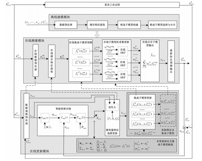
本文提出基于智能更新样本识别算法的在线集成建模策略, 由离线建模、在线测量和在线更新模块三部分组成, 如图 1所示.其中, 离线建模由数据预处理、潜在特征提取、候选子模型构建、集成子模型选择与合并等组成; 在线测量模块由在线数据预处理、在线潜在特征提取、在线集成子模型预测、在线子模型权系数更新及在线合并子模型输出等部分组成; 在线更新模块包括数据递推预处理、智能更新识别、潜变量特征递推更新、集成子模型更新、非更新特征及集成子模型赋值等组成部分.
图 1中, ${{\boldsymbol{x}}}_{k+1}^0 $ 表示未经标定处理的新样本; ${{\pmb x}}_{k+1}^{{\rm old}} $ 表示采用旧均值和方差标定的新样本; ${\pmb z}_{k+1}^{{\rm old}} $ 表示采用旧PLS模型提取的新样本潜在变量; $f_k^{j\ast } (\pmb z_{k+1}^{{\rm old}})$ 和 $\hat {y}_{k+1}^{j\ast {\rm old}} $ 表示新样本基于旧的第 $j^\ast$ 个集成子模型进行预测及其输出; $w_{k+1}^{j\ast } $ 表示基于在线AWF (OLAWF)算法获得的子模型权系数; $\sum_{j\ast=1}^{J\ast } {w_{k+1}^{j\ast } } \hat {y}_{k+1}^{j\ast {\rm old}} $ 表示集成子模型的集成加权计算方法; $J^\ast $ 表示集成子模型数量, 即集成尺寸; $\hat {y}_{k+1} $ 表示新样本基于集成模型的输出; $\hat {y}_{k+1}^0 $ 表示重新标定后的在线测量值; ${{\boldsymbol{x}}}_{k+1} $ 表示数据递推预处理后的新样本; $\pmb z_{k+1}$ 表示潜在变量特征; $\{{{\boldsymbol{x}}}_l \}_{l=1}^k $ 表示旧子模型的建模样本; $f_k^{j\ast } (\pmb z_{k+1})$ 和 $\{(\hat {y}_{k+1}^{j\ast })_l \}_{l=1}^{k+1} $ 表示更新后的第 $j^\ast$ 个集成子模型及其输出; $F_{\rm ALD} (\cdot)$ 、 $F_{{\rm com}} (\cdot)$ 和 $F_{\rm thre} (\cdot)$ 分别表示RALD算法、基于专家规则的模糊融合算法及其决策输出函数; $a_{k+1}$ 表示新样本RALD值; $u_{sk+1}$ 表示融合RALD和RPE的输出值; $\theta _{\rm com} $ 表示基于经验设定的模糊融合输出阈值; $S_{k+1} $ 是更新决策值, 其值为1表示更新, 否则不更新.
该方法不同于其他在线集成模型方法, 集成子模型加权系数的更新是在在线测量阶段通过OLAWF算法完成的, 能够更好地适应工业过程的动态变化.
2.1 离线建模模块
此处采用文献[21]提出的基于潜变量特征的选择性集成IRVFL的建模策略构建离线软测量模型, 主要包括潜变量特征提取、子模型构建、子模型选择和子模型合并4个模块, 如图 2所示.
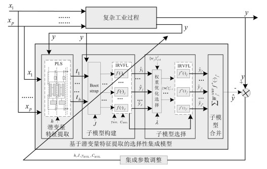 图 2 基于潜变量特征的选择性集成IRVFL离线软测量模型建模策略Fig. 2 Selective ensemble IRVFL off-line soft sensor model based on latent variable features
图 2中, ${{ X}}_k^{{\rm old}}=\{(x_1, \cdots, x_p)_l \}_{l=1}^k $ , 即 $\{{{\boldsymbol{x}}}_l^{{\rm old}} \}_{l=1}^k $ , 表示建模的输入数据集; ${ { Z}}_k^{{\rm old}}=\{(z_1, \cdots $ , $ z_h)_l \}_{l=1}^k $ 表示采用PLS算法提取的潜变量特征, 即选择性集成模型的输入; $\{({ {\pmb z}}_{{\rm sub}}^j, y_{{\rm sub}}^j)_l \}_{l=1}^k $ 表示采用Bootstrap算法产生的第 $j$ 个训练子集; $f(\cdot)_j $ 表示在采用第 $j$ 个训练子集构建的基于IRVFL的候选子模型; $f^\ast (\cdot)_{j^\ast } $ 表示基于遗传算法优化工具箱(GA optimization toolbox, GAOT)选择的第 $j^\ast$ 个集成子模型; $\sum {W_{j^\ast }^{{\rm AWF}} f^\ast (\cdot)_{j^\ast } } $ 表示采用AWF加权算法对集成子模型进行合并; $\hat {y}_j $ 、 $\hat {y}_{j^\ast } $ 和 $\hat {y}$ 分别表示第 $j$ 个候选子模型、第 $j^\ast$ 个集成子模型和集成模型的输出.
由图 2可知, 共有4个学习参数需要选择:潜变量特征个数h、候选子模型数量 $J$ 、IRVFL算法的核参数 $\gamma _{\rm RVFL} $ 和惩罚参数 $C_{\rm RVFL} $ .建立离线选择性集成模型的过程可表述为求解如下优化问题:
$ \begin{matrix} \min {{J}_{\text{RMSRE}}}=\qquad \\ \sqrt{\frac{1}{{{k}^{\text{valid}}}}\sum\limits_{l=1}^{{{k}^{\text{valid}}}}{{{\left(\frac{y_{{}}^{l}-\sum\limits_{{{j}^{*}}=1}^{{{J}^{*}}}{w_{{{j}^{*}}}^{\text{AWF}}}\hat{y}_{{{j}^{*}}}^{l}}{{{y}^{l}}} \right)}^{2}}}} \\ \text{s}.\text{t}.\left\{ \begin{array}{*{35}{l}} {{{\mathbf{\hat{y}}}}_{j}}^{*}=OpSel({{{\mathbf{\hat{y}}}}_{1}}, \cdots, {{{\mathbf{\hat{y}}}}_{j}}, \cdots, {{{\mathbf{\hat{y}}}}_{J}}) \\ {{{\mathbf{\hat{y}}}}_{j}}=f{{\left(\mathbf{z}, {{\gamma }_{\text{IRVFL}}}, {{C}_{\text{IRVFL}}} \right)}_{j}} \\ 2\le {{J}^{*}}\le J \\ 1\le {{j}^{*}}\le {{J}^{*}} \\ 0\le j\le J \\ \sum\limits_{j=1}^{{{J}^{*}}}{w_{{{j}^{*}}}^{\text{AWF}}}=1 \\ 0\le w_{{{j}^{*}}}^{\text{AWF}}\le 1 \\ \end{array} \right. \\ \end{matrix} $
(10) 其中, $J_{{\rm RMSRE}} $ 表示选择性集成模型的均方根相对误差(Root mean square relative error, RMSRE); $k^{\rm valid}$ 表示验证样本集的数量; $OpSel(\cdot)$ 表示集成子模型的优化选择方法; $J^\ast $ 表示优选的集成子模型的数量; $w_{j^\ast }^{\rm AWF} $ 表示优选的集成子模型的加权系数.
PLS分解训练数据 ${ X}_k^{{\rm old}} $ 和 ${ Y}_k^{{\rm old}} $ 提取潜在特征的过程可表示为
$ \begin{matrix} \left[ \begin{matrix} X_{k}^{\text{old}} \\ Y_{k}^{\text{old}} \\ \end{matrix} \right]\Rightarrow \left\{ \begin{array}{*{35}{l}} X_{k}^{\text{old}}=T_{k}^{\text{old}}{{(P_{k}^{\text{old}})}^{\text{T}}}+{{E}_{h}} \\ Y_{k}^{\text{old}}=T_{k}^{\text{old}}B_{k}^{\text{old}}{{(Q_{k}^{\text{old}})}^{\text{T}}}+{{F}_{h}} \\ \end{array} \right.\Rightarrow \text{ } \\ Z_{k}^{\text{old}}=[{{\boldsymbol{t}}_{1}}, {{\boldsymbol{t}}_{2}}, \cdots, {{\boldsymbol{t}}_{h}}] \\ \end{matrix} $
(11) 其中, $T_k^{{\rm{old}}}=[{{\pmb t}_{\rm{1}}}, {{\pmb t}_2}, \cdots, {{\pmb t}_h}]$ , ${{P}}_k^{{\rm{old}}}=[{{\pmb p}_{\rm{1}}}, {{\pmb p}_2}, \cdots$ , ${{\pmb p}_h}]$ , $Q_k^{{\rm{old}}}=[{{\pmb q}_{\rm{1}}}, {{\pmb q}_2}, \cdots, {{\pmb q}_h}]$ , $B_k^{{\rm{old}}}={\rm diag}\{ {b_{\rm{1}}}, {b_2}$ , $\cdots$ , ${b_h}\} $ 分别表示由训练数据分解得到的得分矩阵、输入数据负荷矩阵、输出数据负荷矩阵和PLS内部模型的系数矩阵.
采用Bootstrap算法基于提取的潜在特征矩阵产生的训练子集, 即
$ Z_k^{{\rm{old}}}=\{ {({{\pmb z}}, y)_l}\} _{l=1}^k \Rightarrow {\begin{cases} {\{ {{({{\pmb z}}_{{\rm{sub}}}^1, y_{{\rm{sub}}}^1)}_l}\} _{l=1}^k}\\ \qquad\quad{\vdots}\\ {\{ {{({{\pmb z}}_{{\rm{sub}}}^j, y_{{\rm{sub}}}^j)}_l}\} _{l=1}^k}\\ \qquad\quad{\vdots}\\ {\{ {{({{\pmb z}}_{{\rm{sub}}}^J, y_{{\rm{sub}}}^J)}_l}\} _{l=1}^k} \end{cases}} $
(12) 其中, $J$ 是训练子集的数量, 即候选子模型的数量.
采用核矩阵 $ K_j ({\pmb z}_l, {\pmb z}_m)$ 替代RVFL的隐含层特征映射 ${ {{\pmb h}({\pmb z})}}$ , RVFL算法针对第 $j$ 个候选子模型的输出可表示为
$ f_k^j({{\pmb z}})={\pmb h}({\pmb z}){H}^{\rm{T}}\left(\frac{{\rm I}}{{C_{\rm{RVFL}}}} + H{H}^{\rm{T}} \right)^{-1}\\Y=[{K}_j({\pmb z}, {{\pmb z}_1}), {K}_j({\pmb z}, {{\pmb z}_2}), \cdots, {K}_j({\pmb z}, {{\pmb z}_k})]\, \times \\ \left(\frac{{I}}{{C{}_{{\rm{RVFL}}}}} + {K}_j({{\pmb z}_l}, {{\pmb z}_m}) \right)^{-1}Y $
(13) 其中, $H$ 是RVFL的隐含层矩阵.
从构建的 $J$ 个候选子模型选择 $J^\ast $ 个集成子模型的过程可表示为
$ \left. {\begin{array}{*{20}{l}} {\{ f_k^j(\cdot)\} _{j=1}^J }\\[2mm] {\{ {w_j}\} _{j=1}^J } \end{array}} \right\} \Rightarrow {\rm{GAOT}} \Rightarrow \left\{ {\begin{array}{*{20}{l}} {\{ f_k^{j*}(\cdot)\} _{{j^*}=1}^{{J^*}}}\\[2mm] {\{ {w_{{j^*}}}\} _{{j^*}=1}^{{J^*}}}~~~\end{array}} \right. $
(14) 对选择的集成子模型基于AWF算法计算权重系数, 并采用 $\sum {W_{j^\ast }^{\rm AWF} f^\ast (\cdot)_{j^\ast } } $ 合并集成子模型的输出 $\hat {y}_{j^\ast } $ , 即得到最终选择性集成模型的输出 $\hat {y}$ .
由以上离线建模过程可知, 本文建立的选择集成模型采用``采集训练样本''的方式产生训练子集并构建选择性集成模型, 并非工业工程常用多模型建模策略所采用的``聚类算法获得代表不同工况的训练样本构建集成子模型再集成的策略''; 此外, 本文采用SVM核矩阵替代RVFL的隐含层映射, 输入权重的随机性得到抑制.因此, 对集成模型的学习参数进行更新是必要的.另外, 无论采用何种方式产生训练子集, 只要过程对象漂移产生的新工况在建模样本覆盖范围之外, 都有必要对集成模型的结构和参数同时进行更新.
2.2 在线测量模块
在线数据预处理时, 新样本采用旧均值和方差进行标定
$ {\boldsymbol{x}}_{k + 1}^{{\rm{old}}}=\left({\boldsymbol{x}}_{k + 1}^0-{{{\pmb 1}}_k}{{\pmb u}}_k^{\rm{T}}\right) \times \Sigma_k $
(15) 其中, ${\pmb u}_k^{}$ 和 $\Sigma_k^{}$ 表示旧建模数据 $\{ {\pmb x}_l^{{\rm{old}}}\} _{l=1}^k$ 的均值和标准差.
为表述方便, 将离线阶段基于建模样本 $\{ {\boldsymbol{x}}_l^{{\rm{old}}}\} _{l=1}^k$ 和 $\{ y_l^{{\rm{old}}}\} _{l=1}^k$ 建立的PLS模型表示为
$ left\{ {\{ {\boldsymbol{x}}_l^{{\rm{old}}}\} _{l=1}^k, \{ y_l^{{\rm{old}}}\} _{l=1}^k} \Rightarrow {\rm{PLS}} \Rightarrow \\ \left\{ T_k^{\rm{old}}, W_k^{\rm{old}}, P_k^{\rm{old}}, B_k^{\rm{old}}, Q_k^{\rm{old}} \right\} $
(16) 基于 ${\boldsymbol{x}}_{k + 1}^{\rm{old}}$ 提取的潜在特征可表示为
$ {\pmb z}_{k + 1}^{\rm{old}}={\boldsymbol{x}}_{k + 1}^{\rm{old}}W_k^{\rm{old}}\left({{{{\rm{(}}{{P}}_k^{{\rm{old}}})}^{\rm{T}}}W_k^{{\rm{old}}}} \right)^{-1} $
(17) 其中, ${\pmb z}_{k + 1}^{\rm{old}}$ 表示潜在特征; $P_k^{\rm{old}}$ 和 $W_k^{{\rm{old}}}$ 是旧PLS模型的负荷和系数矩阵.
新样本基于第 $j$ 个旧集成子模型的预测输出
$ \hat y_{k + 1}^{j*{\rm{old}}}=f_k^{j*}\left({\pmb z}_{k + 1}^{{\rm{old}}}\right) $
(18) 其中, $f_k^{j*}(\cdot)$ 表示第 $j$ 个旧集成子模型.
采用在线AWF算法计算集成子模型权系数[3]
$ u_{k + 1}^{j*}=\frac{k}{{k + 1}}u_k^{j*{\rm{old}}} + \frac{1}{{k + 1}}\hat y_{k + 1}^{j*{\rm{old}}} $
(19) $ {\left(\sigma _{k + 1}^{j*}\right)^2}=\dfrac{{k-1}}{k}{\left(\sigma _k^{j*{\rm{old}}}\right)^2} + {\left(u_{k + 1}^{j*{\rm{old}}}-u_k^{j*{\rm{old}}}\right)^2~}+ \dfrac{1}{k}\|\hat y_{k + 1}^{j*}-u_{k + 1}^{j*}\|^2 $
(20) $ w_{k + 1}^{j*}=\frac{1} {\left(\sigma_{k + 1}^{j*}\right)^2\sum\limits_{j^*=1}^{J^*} {\frac{1}{\left(\sigma _{k + 1}^{j*}\right)^2 } }} $
(21) 其中, $u_{k + 1}^{j*}$ , $\sigma _{k + 1}^{j*}$ 及 $w_{k + 1}^{j*}$ 分别表示更新后的均值、方差及子模型权系数.
新样本的在线测量输出 $\hat y_{k + 1}^{}$ 采用下式计算:
$ \hat y_{k + 1}^{}=\sum\limits_{j*=1}^{J*} {w_{k + 1}^{j*}} \hat y_{k + 1}^{j*} $
(22) 采用旧模型标定参数对 $\hat y_{k + 1}^{}$ 进行重新标定:
$ \hat y_{k + 1}^0=A + \frac{{(\hat y_{k + 1}^{}-0.1)(A-B)}}{{0.9-0.1}} $
(23) 其中, $A$ 和 $B$ 为旧建模样本 $\{ y_l^{{\rm{old}}}\} _{l=1}^k$ 中的最小值和最大值.
2.3 在线更新模块
通常, 获得 $k+1$ 时刻真值后进行模型更新, 因而在 $k+1$ 时刻更新的模型只能在 $k+2$ 时刻进行基于软测量模型的在线测量输出.
2.3.1 数据递推预处理
在线数据预处理需考虑新样本对旧建模样本的均值和方差的影响.首先对旧建模样本的均值和方差进行递推更新
$ {{\pmb u}_{k + 1}}=\frac{k}{{k + 1}}{{\pmb u}_k} + \frac{1}{{k + 1}}{\left({\boldsymbol{x}}_{k + 1}^0\right)^{\rm{T}}} $
(24) $ \sigma _{(k + 1) \cdot {i_p}}^2=\frac{{k-1}}{k}\sigma _{k \cdot {i_p}}^2 + \Delta {\pmb u}_{k + 1}^2\left({i_p}\right)~+\nonumber\\ \frac{1}{k}{\left\| {{\boldsymbol{x}}_{k + 1}^0({i_p})-{{\pmb u}_{k + 1}}({i_p})} \right\|^2} $
(25) 其中, $\Delta {\pmb u}_{k + 1}^{}={\pmb u}_{k + 1}^{}-{\pmb u}_k^{}$ ; $\sigma _{(k + 1) \cdot {i_p}}^{}$ 表示第 $i_p$ 个变量的标准差.
新样本标定的递推形式为
$ {{\boldsymbol{x}}_{k + 1}}=({\boldsymbol{x}}_{k + 1}^0-{\bf{1}} \cdot {\pmb u}_{k + 1}^{\rm{T}}) \times \Sigma _{k + 1} $
(26) 其中, ${\Sigma _{k + 1}}={\rm diag}\{{\sigma _{(k + 1){1_p}}}, \cdots, {\sigma _{(k + 1){p_p}}}\}$ .
采用与 ${\boldsymbol{x}}_{k + 1}^0$ 相同的方法预处理 $y_{k + 1}^0$ , 并将标定后的值记为 $y_{k + 1}^{}$ .
2.3.2 更新样本智能识别
更新样本智能识别中同时考虑新样本ALD值和PE值的影响.基于领域专家知识总结规则, 建立基于Mamdani模糊推理系统的智能模型对ALD值和PE值进行融合输出.
采用文献[8]的方法计算 ${{\boldsymbol{x}}}_{k+1} $ 相对于建模样本库的ALD绝对值 $a_{k + 1}^{\rm{abs}}$ .
$ \begin{cases} a_{k + 1}^{{\rm{abs}}}={k_{k + 1}}-{{\left({\tilde{\pmb k}}_k^{}\right)}^{\rm{T}}}{{\left({{\tilde K}}_k^{}\right)}^{-1}}\left({\tilde{\pmb k}}_k\right)\\[1mm] {\tilde K}_k=X_k^{\rm{old}} \times \left(X_k^{\rm{old}}\right)^{\rm{T}}\\[1mm] \tilde{\pmb k}_k=X_k^{\rm{old}} \times {\boldsymbol{x}}_{k + 1}^{\rm{T}} \\[1mm] k_{k + 1}={\boldsymbol{x}}_{k + 1} \times {\boldsymbol{x}}_{k + 1}^{\rm{T}} \end{cases} $
(27) 其中, $X_k^{\rm{old}}$ 表示旧的建模样本数据集.
计算新样本的相对ALD (RALD)值 $a_{k + 1}^{}$ :
$ a_{k + 1}=\dfrac{a_{k + 1}^{\rm abs}} {\frac{\sum\limits_{l=1}^{k } a_l^{\rm abs}} {k}} $
(28) 其中, $a_l^{{\rm{abs}}}$ 表示建模样本库中第 $l$ 个样本相对于其他所有 $k-1$ 个样本的ALD值.
上述过程可采用如下公式表示:
$ a_{k + 1}^{}=F_{{\rm{ALD}}}^{}\left({\boldsymbol{x}}_{k + 1}^{}, \{ {\pmb x}_l^{{\rm{old}}}\} _{l=1}^k\right) $
(29) 考虑 $k+1$ 时刻PE值的影响, 定义相对预测误差(RPE)如下:
$ e_{k + 1}=\dfrac{\left| \dfrac{\hat y_{k + 1}-y_{k + 1}}{y_{k + 1}} \right|} {\frac {\sum\limits_{l=1}^k {\left| \dfrac{\hat y_l-y_l}{y_l} \right|}}{k} } $
(30) 其中, $\left| {\frac{{\hat y_{k + 1}^{}-y_{k + 1}^{}}}{{y_{k + 1}^{}}}} \right|$ 表示建模样本库第 $l$ 个样本的预测值与其真值的相对差值.
此处将融合新样本RPE和RALD值建立的更新样本智能识别算法记为 $F_{{\rm{com}}}^{}(\cdot)$ , 并将智能识别算法的输出称为模糊融合值, 记为 ${u_s}_{k +1}^{}$ , 用下式表示:
$ u_{sk + 1}^{}=F_{{\rm{com}}}^{}(a_{k + 1}^{}, e_{k + 1}^{}) $
(31) 采用基于专家经验总结的模糊推理规则实现对RALD值和RPE值的融合输出, 参考PID控制器设计的比例-积分控制律, 总结如表 1所示49条专家规则.
表 1 更新样本模糊推理规则Table 1 Fuzzy inference rulers of the updating sampleUs RALD NB NM NS Z PS PM PB R NB NB NB NM NM NS NS Z P NM NB NM NM NS NS Z PS E NS NM NM NS NS Z PS PS Z NM NS NS Z PS PS PM PS NS NS Z PS PS PM PM PM NS Z PS PS PM PM PB PB Z PS PS PM PM PB PB 表 1中, RALD、RPE和Us分别表示新样本面对旧建模样本库的相对近似线性依靠值、新样本基于旧模型的相对预测误差值和模糊融合值.
采用重心法对Us进行去模糊处理.将样本选择阈值记为 $\theta _{{\rm com}} $ , 阈值函数 ${F_{{\rm{thre}}}}(\cdot)$ 可记为
$ S_{k + 1}^{}={F_{{\rm{thre}}}}\left(c_{k + 1}^{}, \theta _{{\rm{com}}}\right)=\begin{cases} 1, & {u_s}_{k + 1} \ge \theta _{\rm{com}}\\ 0, & {u_s}_{k + 1}^{} < \theta _{\rm{com}} \end{cases} $
(32) 其中, $S_{k + 1}=1$ 表示识别该新样本为更新样本.
2.3.3 潜变量特征递推更新
将标定后的新样本记为 $\{ {{\boldsymbol{x}}_{k + 1}^{}, {{ y}}_{k + 1}^{}} \}$ 进行递推更新的输入输出数据可记为
$ {X}_{k + 1}=\left[{\begin{array}{*{20}{c}} {{{({{P}}_k^{\rm{old}})}^{\rm{T}}}}\\ {{{\boldsymbol{x}}_{k + 1}}} \end{array}} \right]\notag\\[2mm] {Y}_{k + 1}=\left[\begin{array}{*{20}{c}} {B}_k^{\rm{old}}{(Q_k^{\rm{old}})}^{\rm{T}}\\ {{{{ y}}_{k + 1}}} \end{array} \right] $
(33) 基于以上输入输出数据建立新PLS模型
$ \begin{matrix} \left\{ {{X}_{k+1}}, {{Y}_{k+1}} \right\}\Rightarrow \text{PLS}\Rightarrow \\ \left\{ {{T}_{k+1}}, {{W}_{k+1}}, {{P}_{k+1}}, {{B}_{k+1}}, {{Q}_{k+1}} \right\} \\ \end{matrix} $
(34) 基于 ${{\boldsymbol{x}}}_{k+1} $ 提取的潜在特征可表示为
$ {{\pmb z}}_{k + 1}={\boldsymbol{x}}_{k + 1}W_k\left({{({{P}}_k)}^{\rm{T}}}W_k \right)^{-1} $
(35) 其中, ${\pmb z}_{k + 1}$ 表示新样本的潜在特征; ${P}_{k + 1}$ 和 $W_{k + 1}$ 是新PLS模型的负荷矩阵和系数矩阵.
2.3.4 集成子模型更新
确定采用子模型更新时, 建模样本集为
$ \{ {{{\pmb z}}_l}, {y_l}\} _{l=1}^{k + 1}=\{ {{{\pmb z}}_l}, {y_l}\} _{l=1}^k \cup \{ {{\pmb z}}_{k + 1}^{}, {{ y}}_{k + 1}^{}\} $
(36) 因IRVFL算法具有较快的学习速度, 此处采用新建模样本库重新训练方式进行集成模型更新.更新后的集成子模型 $f_{k + 1}^{j*}(\cdot)$ 对训练样本的输出为
$ \{ {(\hat y_{k + 1}^{j*})_l}\} _{l=1}^{k + 1}=f_{k + 1}^{j*}(\{ {{{\pmb z}}_l}\} _{l=1}^{k + 1}) $
(37) 为保证采集到第 $(k+2)$ 个新样本时在线测量模块可以正常运行, 需更新的变量及模型包括:建模样本的均值 ${\pmb u}_{k + 1}$ 和标准差 $\Sigma_{k + 1}$ , 潜变量特征提取模型的 $B_k$ , $Q_k$ , ${{P}}_{k + 1}$ 和 $W_{k + 1}$ , 集成子模型 $f_{k + 1}^{j*}(\cdot)$ , 集成子模型预测值的均值 $u_{k + 1}^{j*}$ 和方差 $\sigma _{k + 1}^{j*}$ .按如下公式进行赋值:
$ \begin{cases} {\pmb u}_{k + 1}^{} \leftarrow {\pmb u}_k\\ \Sigma_{k + 1} \leftarrow \Sigma_k \end{cases} $
(38) $ \begin{cases} {P}_{k + 1}^{} \leftarrow {{P}}_k\\ B_{k + 1} \leftarrow B_k\\ W_{k +1 } \leftarrow W_k\\ {Q}_{k + 1} \leftarrow Q_k \end{cases} $
(39) $ f_{k + 1}^{j*}(\cdot) \leftarrow f_k^{j*}(\cdot) $
(40) $ \begin{cases} u_{k + 1}^{j*} \leftarrow u_k^{j*}\\ \sigma _{k + 1}^{j*} \leftarrow \sigma _k^{j*} \end{cases} $
(41) 3. 仿真验证
采用如下函数生成仿真数据模拟工业过程的非线性和时变特性:
$ \begin{cases} {{x_1}={t^2}-t + 1 + {\Delta _1}}~~~~~~~~~~~~~~~~~~~~~~~~~~~~~~~~~~~\\ {{x_2}=\sin (t) + {\Delta _2}}~~~~~~~~~~~~~~~~~~~~~~~~~~~~~~~~~~~~~~~~~~\\ {{x_3}={t^3} + t + {\Delta _3}}~~~~~~~~~~~~~~~~~~~~~~~~~~~~~~~~~~~~~~~~~~\\ {{x_4}={t^3} + {t^2} + 1 + {\Delta _4}}~~~~~~~~~~~~~~~~~~~~~~~~~~~~~~~~~~\\ {{x_5}=\sin (t) + 2{t^2} + 2 + {\Delta _5}}~~~~~~~~~~~~~~~~~~~~~~~~~~~~~\\ {y=x_1^2 + x_1^{}{x_2} + 3\cos {x_3}-{x_4} + 5{x_5} + {\Delta _6}} \end{cases} $
(42) 其中, $t\in [-1, 1]$ , $\Delta _{i_{{\rm sy}} } $ 表示噪声, 其分布范围为[-0.1,0.1], $i_{{\rm sy}}=1, 2, 3, 4, 5, 6$ .
仿真合成数据分布在 $C1$ 、 $C2$ 、 $C3$ 和 $C4$ 共4个不同区域.训练样本数量由分别来自 $C1$ 、 $C2$ 和 $C3$ 区域的各30个样本组成.测试样本由 $C1$ 、 $C2$ 和 $C3$ 区域的各30个样本以及 $C4$ 区域的90个样本组成.
3.1 离线模型结果
基于90个训练样本, 采用PLS进行特征提取, 不同LV的方差贡献率如表 2所示.
表 2 仿真数据的方差贡献率(%)Table 2 Percent variance contribution of the simulation data(%)LV 输入数据(X-Block) 输出数据(Y-Block) 潜变量贡献率 累计贡献率 潜变量贡献率 累计贡献率 1 69.79 69.79 66 66 2 28.33 98.11 25.66 91.65 3 1.62 99.73 7.86 99.51 4 0.16 99.89 0.05 99.56 5 0.11 100 0 99.57 表 2表明, 前3个LVs分别描述了 $X$ -Block和 $Y$ -Block方差变化率的99.73, %和99.51, %.不同模型学习参数(核半径、惩罚参数、候选子模型数量、潜变量数量)与均方根预测相对误差(RMSRE)间的关系如图 3所示.
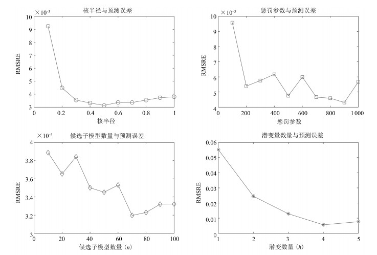 图 3 离线模型学习参数与预测误差Fig. 3 Learning parameters and prediction errors of the off-line model
依据图 3进行建模参数选择.为便于比较, 将RALD值和RPE值采用极差法标定在 $-3$ 与 $+3$ 之间, 测试样本相对于初始建模样本的RALD值、\linebreak RPE值及模糊融合值如图 4所示.
 图 4 测试样本相对于离线模型(建模样本)的RALD值、RPE值及模糊融合值Fig. 4 RALD, RPE and fuzzy fusion values of the testing samples relative to off-line model (modeling samples)
由图 4可知, 后90个测试样本相对于建模样本的变化高于前90个测试样本, 主要原因是后90个样本代表的新的概念漂移未能被初始建模样本所覆盖; 以阈值0为界限, 由位于阈值线上方的样本分布可知, 所提更新样本识别算法可有效地融合RALD值和RPE值.由上可知, 进行集成模型的在线更新非常必要.
3.2 在线模型结果
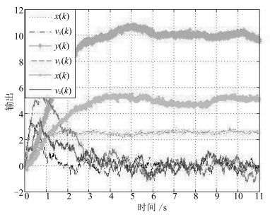
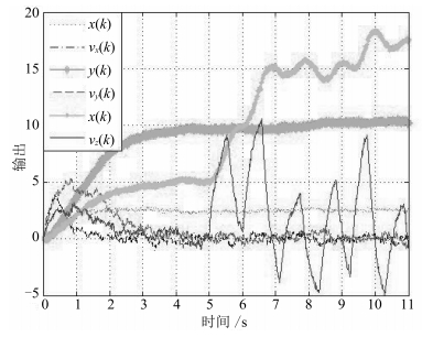
模糊融合阈值 $\theta _{{\rm com}}$ 的大小决定了模型更新次数的多少, 较大的阈值代表更多的样本参与更新.本文将阈值的取值范围定为 $-3$ ~ $+3$ 之间.当 $\theta _{{\rm com}}=$ $-1.5$ 时, 测试样本相对于在线更新模型建模样本的RALD值、在线更新模型的RPE值、对两者融合的模糊融合值及在线更新模型的测试曲线, 如图 5所示.表 3给出了离线模型, 基于RALD值、RPE值和模糊融合值的在线更新模型重复20次的统计结果.
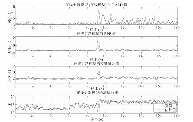 图 5 $\theta _{{\rm com}}=-1.5$ 时的在线集成模型预测输出Fig. 5 Prediction output of the online ensemble model with $\theta _{{\rm com}}=-1.5 $表 3 仿真数据在线更新模型重复20次的统计结果Table 3 Statistical results of the online updating model with repeated 20 times for the simulation data
更新样本识别方法 统计项 更新样本预设定阈值 –2.5 –2 –1.5 –1 0 1 非更新方法 最大误差 0.1886 0.1885 0.1884 0.1894 0.1887 0.1892 最小误差 0.1875 0.1865 0.187 0.1872 0.1872 0.1871 误差均值 0.1868 0.1876 0.1878 0.1879 0.1878 0.1879 误差方差 0.0004 0.0004 0.0004 0.0005 0.0004 0.0005 基于RALD的更新样本识别方法 最大误差 0.1758 0.1152 0.0989 0.1127 0.1004 0.1767 最小误差 0.0628 0.0794 0.0856 0.085 0.087 0.1658 误差均值 0.119 0.0876 0.0892 0.0886 0.0911 0.1878 误差方差 0.0376 0.0094 0.0044 0.006 0.0033 0.0071 更新次数最多的样本编号 92, 94, 96, 118, 119, 141 99, 100, 106, 98, 100, 103 99, 106, 118, 124 99, 106 99, 123, 149, 154 - 平均更新次数 11 5 2 2 2 0 基于RPE的更新样本识别方法 最大误差 0.058 0.0665 0.0486 0.085 0.1198 0.1701 最小误差 0.0396 0.038 0.0449 0.05 0.0492 0.0494 误差均值 0.044 0.0446 0.0469 0.0642 0.0785 0.0731 误差方差 0.0042 0.007 0.0008 0.012 0.0231 0.0284 更新次数最多的样本编号 91, 92, 93, 118, 124 91, 93, 92, 97, 95 91, 93, 1 91, 93, 8, 1, 119 91, 93, 8, 16, 11 93, 91, 92, 11 平均更新次数 10.3 4.1 2.05 2.6 2.2 1.9 本文方法 最大误差 0.16 0.0953 0.0733 0.0808 0.1082 0.1878 最小误差 0.0967 0.0529 0.0397 0.0395 0.0556 0.1653 误差均值 0.1309 0.0784 0.0429 0.0474 0.0847 0.1804 误差方差 0.0199 0.0116 0.0078 0.0101 0.0117 0.0066 更新次数最多的样本编号 1180 91, 91, 93, 95, 97, 76 91, 92, 93, 97, 124 93, 91, 92 92, 94, 93, 99 – 平均更新次数 180 72.95 3.4 2.55 1.7 0 1) 从更新最多的样本编号上看, 本文方法选择的样本基本上覆盖了RALD和RPE方法选择的样本, 如依据RALD方法未选择的第93和97个样本、依据RPE方法未选择的第99和106个样本在本文所提模糊融合方法中均进行了选择, 表明该方法可以有效地融合RALD和RPE方法中独立存在的片面信息.
2) 在模型预测性能上, 不同更新阈值时的不同更新方法的最大、最小和平均预测误差如图 6所示.
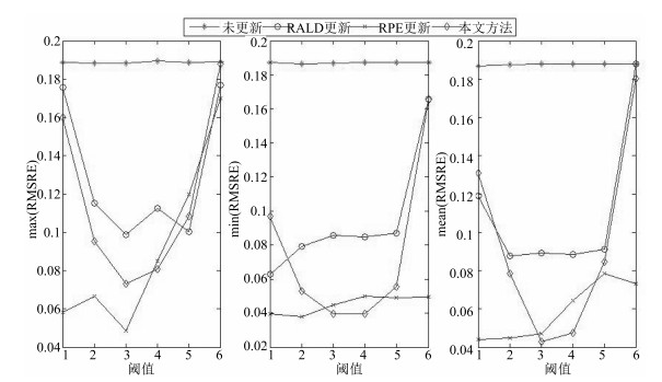 图 6 基于不同更新样本识别方法软测量模型的预测误差Fig. 6 Prediction errors of the soft sensor models based on different updating sample identification methods
图 6表明, 未更新时软测量模型具有最差的泛化性能, 主要是因为离线模型不能适应 $C4$ 区域所表征的新工况; 对于基于RALD、基于RPE和本文所提方法更新的软测量模型的预测性能均有一定程度的提高.在阈值取 $-1.5$ 时, 基于RPE的方法具有最佳的最大预测误差, 本文方法具有最佳的最小和平均预测误差.如, 基于本文、RPE和RALD方法的平均RMSRE分别为0.0429、0.0469和0.0892, 方差分别为0.0078、0.0008和0.0044.
图 6还表明, 从曲线形状的角度观察, 本文所提方法的预测误差说明存在最佳的阈值能够使软测量模型具有最佳预测性能.
3) 在更新样本数量上, 本文方法与基于RALD和RPE方法相当, 如在样本更新阈值为 $-1.5$ 时, 基于本文方法、RPE方法和RALD方法的重复20次的平均更新样本数量分别3.4、2.05和2, 表明三种方法均只需采用较少数量的更新样本即可得到较佳预测性能, 原因之一在于每次样本更新后均是重新建立集成子模型, 对集成模型的结构、权重系数等均进行了更新; 不足之处是未对集成子模型的超参数(如核半径)进行更新.如何在线更新模型超参数将进一步研究, 以便提高模型的泛化性能.
4) 从不同阈值的影响上看, 理论上阈值越小, 模型的预测性能越好, 即参与更新的样本越多模型预测误差越小; 当更新样本数量累计过多时模型的预测性能提高较小, 甚至反而下降, 这是因为过多与临近工作点无关的样本恶化了模型预测性能.下步研究中将考虑如何识别和删减恶化模型性能的多余样本.
5) 本文方法与文献[9]提出的在线KPLS方法相比, 模型更新次数明显减少, 主要原因在于本文所提方法更新了模型结构, 进一步表明集成模型结构在线更新的必要性和有效性.
综上, 本文方法对具有明确时变特性的建模过程数据是有效的.需提出的是, 模糊规则的调整需要领域专家依据具体建模对象特性、软测量模型性能及其他难以量化的因素等综合确定.在后续研究中, 需要结合真实的时变工业过程数据进行进一步的细化研究.
4. 结论
本文提出的在线更新学习中, 模型更新次数是通过模糊规则融合新样本的相对近似线性依靠值和相对预测误差值确定的.智能识别模型的模糊规则主要是依靠领域专家经验确定, 在实际应用中需要结合具体的工业过程应用对象进行提取, 并提供可供调整的人机交互界面.另外, 主要关注更新样本近似线性依靠条件, 还是预测误差所表征的概念漂移可通过调整隶属度函数进一步细划.因此, 该方法能够有效地实现更新样本的智能识别, 通过合理设定模糊推理规则能够在集成模型预测性能与更新效率之间进行均衡, 结合具体工程应用将具有广阔前景.
本文方法进行近似线性依靠条件计算需要记录全部训练样本, 更新集成模型也需要存储建立核矩阵的潜在特征, 导致集成模型存储的数量逐渐递增.集成模型的快速递推更新、模型超参数的快速优化选择等问题将在后续研究中逐步解决.
-
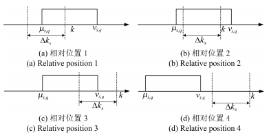
图 1 间歇故障与滑动时间窗口的相对位置关系
Fig. 1 Relative positions between the intermittent fault and the sliding-time windo
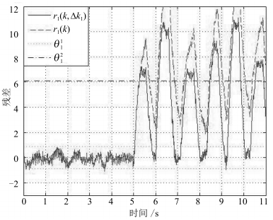
图 4 初始残差信号 $r_1(k)$ 和新残差信号 $r_1(k, \Delta k_1)$
Fig. 4 Comparing $r_1(k, \Delta k_1)$ with $r_1(k)$
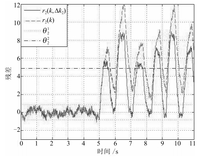
图 5 初始残差信号 $r_2(k)$ 和新残差信号 $r_2(k, \Delta k_2) $
Fig. 5 Comparing $r_2(k, \Delta k_2)$ with $r_2(k)$
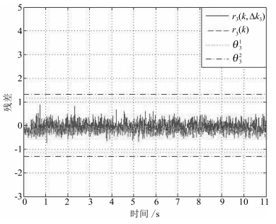
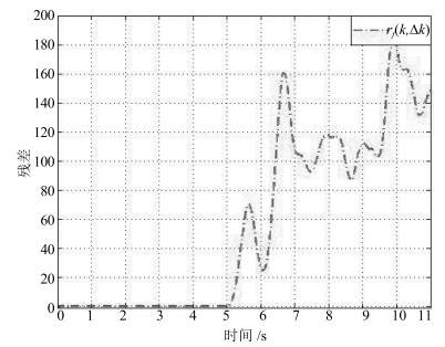
图 6 初始残差信号 $r_3(k)$ 和新残差信号 $r_3(k, \Delta k_3) $
Fig. 6 Comparing $r_3(k, \Delta k_3)$ with $r_3(k)$
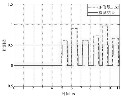
表 1 间歇故障发生(消失)时刻及其实际检测值
Table 1 The detection result of $m_3(k)$ by using the proposed method
q $\mu_{3, q}$ $\mu_{3, q}^{\text{dec}}$ $\nu_{3, q}$ $\nu_{3, q}^{\text{dec}}$ 1 5.00 5.03 5.57 5.62 2 6.02 6.03 6.59 6.67 3 7.14 7.15 7.75 7.77 4 8.32 8.34 8.83 8.87 5 9.26 9.28 9.76 9.87  下载: 导出CSV
-
[1] 周东华, 史建涛, 何潇.动态系统间歇故障诊断技术综述.自动化学报, 2014, 40(2):161-171 http://www.aas.net.cn/CN/abstract/abstract18279.shtmlZhou Dong-Hua, Shi Jian-Tao, He Xiao. Review of intermittent fault diagnosis techniques for dynamic systems. Acta Automatica Sinica, 2014, 40(2):161-171 http://www.aas.net.cn/CN/abstract/abstract18279.shtml [2] Chen M Y, Xu G B, Yan R Y, Ding S X, Zhou D H. Detecting scalar intermittent faults in linear stochastic dynamic systems. International Journal of Systems Science, 2015, 46(8):1337-1348 http://cn.bing.com/academic/profile?id=2005939068&encoded=0&v=paper_preview&mkt=zh-cn [3] Correcher A, García E, Morant F, Quiles E, Blasco-Gimenez R. Intermittent failure diagnosis in industrial processes. In:Proceedings of the 2003 IEEE International Symposium on Industrial Electronics. Rio de Janeiro, Brazil:IEEE, 2003. 723-728 [4] Rashid L, Pattabiraman K, Gopalakrishnan S. Characterizing the impact of intermittent hardware faults on programs. IEEE Transactions on Reliability, 2015, 64(1):297-310 doi: 10.1109/TR.2014.2363152 [5] Shivakumar P, Kistler M, Keckler S W, Burger D, Alvisi L. Modeling the impact of device and pipeline scaling on the soft error rate of processor elements. Computer Science Department, University of Texas at Austin, 2002. http://cn.bing.com/academic/profile?id=87137010&encoded=0&v=paper_preview&mkt=zh-cn [6] 周东华, 魏慕恒, 司小胜.工业过程异常检测、寿命预测与维修决策的研究进展.自动化学报, 2013, 39(6):711-722 http://www.aas.net.cn/CN/abstract/abstract18097.shtmlZhou Dong-Hua, Wei Mu-Heng, Si Xiao-Sheng. A survey on anomaly detection, life prediction and maintenance decision for industrial processes. Acta Automatica Sinica, 2013, 39(6):711-722 http://www.aas.net.cn/CN/abstract/abstract18097.shtml [7] Sorensen B A, Kelly G, Sajecki A, Sorensen P W. An analyzer for detecting intermittent faults in electronic devices. In:Proceedings of AUTOTESTCON'94 IEEE Conference on Systems Readiness Technology——"Cost Effective Support into the Next Century". Anaheim, USA:IEEE, 1994. 417-421 [8] Yesilyurt I, Gu F S, Ball A D. Gear tooth stiffness reduction measurement using modal analysis and its use in wear fault severity assessment of spur gears. NDT and E International, 2003, 36(5):357-372 doi: 10.1016/S0963-8695(03)00011-2 [9] Zanardelli W G, Strangas E G, Aviyente S. Identification of intermittent electrical and mechanical faults in permanent-magnet AC drives based on time-frequency analysis. IEEE Transactions on Industry Applications, 2007, 43(4):971-980 doi: 10.1109/TIA.2007.900446 [10] 马洁, 李刚, 陈默.基于非线性故障重构的旋转机械故障预测方法.自动化学报, 2014, 40(9):2045-2049 http://www.aas.net.cn/CN/abstract/abstract18477.shtmlMa Jie, Li Gang, Chen Mo. Nonlinear fault reconstruction based fault prognosis for rotating machinery. Acta Automatica Sinica, 2014, 40(9):2045-2049 http://www.aas.net.cn/CN/abstract/abstract18477.shtml [11] Hamel A, Gaudreau A, Cote M. Intermittent arcing fault on underground low-voltage cables. IEEE Transactions on Power Delivery, 2004, 19(4):1862-1868 doi: 10.1109/TPWRD.2003.822979 [12] Correcher A, García E, Morant F, Quiles E, Rodriguez L. Intermittent failure dynamics characterization. IEEE Transactions on Reliability, 2012, 61(3):649-658 doi: 10.1109/TR.2012.2208300 [13] Kim C J. Electromagnetic radiation behavior of low-voltage arcing fault. IEEE Transactions on Power Delivery, 2009, 24(1):416-423 doi: 10.1109/TPWRD.2008.2002873 [14] 周东华, 陈茂银, 徐正国.可靠性预测与最优维护技术.合肥:中国科学技术大学出版社, 2013.Zhou Dong-Hua, Chen Mao-Yin, Xu Zheng-Guo. The Reliabibility Prediction and Optimal Maintenance Technology. Hefei:Press of University of Science and Technology of China, 2013. [15] 徐贵斌.动态系统故障诊断及预测研究[硕士学位论文], 清华大学, 中国, 2011.Xu Gui-Bin. Researches on Fault Diagnosis and Prediction in Dynamic Systems[Master dissertation], Tsinghua University, China, 2011. [16] Krasnobaev V A, Krasnobaev L A. Application of Petri nets for the modeling of detection and location of intermittent faults in computers. Automation and Remote Control, 1989, 49(9):1198-1204 [17] Bennett S M, Patton R J, Daley S, Newton D A. Torque and flux estimation for a rail traction system in the presence of intermittent sensor faults. In:Proceedings of United Kingdom Automatic Control Council International Conference on Control'96. Exeter University, UK:IET, 1996. 72-77 [18] Wang Y, Xu G H, Zhang Q, Liu D, Jiang K S. Rotating speed isolation and its application to rolling element bearing fault diagnosis under large speed variation conditions. Journal of Sound and Vibration, 2015, 348:381-396 doi: 10.1016/j.jsv.2015.03.018 [19] Zhou C J, Huang X F, Xiong N X, Qin Y Q, Huang S. A class of general transient faults propagation analysis for networked control systems. IEEE Transactions on Systems, Man, and Cybernetics:Systems, 2015, 45(4):647-661 doi: 10.1109/TSMC.2014.2384480 [20] 顾洲, 张建华, 杜黎龙.一类具有间歇性执行器故障的时滞系统的容错控制.控制与决策, 2011, 26(12):1829-1834 http://www.cnki.com.cn/Article/CJFDTOTAL-KZYC201112014.htmGu Zhou, Zhang Jian-Hua, Du Li-Long. Fault tolerant control for a class of time-delay systems with intermittent actuators failure. Control and Decision, 2011, 26(12):1829-1834 http://www.cnki.com.cn/Article/CJFDTOTAL-KZYC201112014.htm [21] Edelmayer A, Bokor J, Szigeti F, Keviczky L. Robust detection filter design in the presence of time-varying system perturbations. Automatica, 1997, 33(3):471-475 doi: 10.1016/S0005-1098(96)00189-6 [22] Kudva P, Viswanadham N, Ramakrishna A. Observers for linear systems with unknown inputs. IEEE Transactions on Automatic Control, 1980, 25(1):113-115 doi: 10.1109/TAC.1980.1102245 [23] Meskin N, Khorasani K. Fault detection and isolation of discrete-time Markovian jump linear systems with application to a network of multi-agent systems having imperfect communication channels. Automatica, 2009, 45(9):2032-2040 doi: 10.1016/j.automatica.2009.04.020 期刊类型引用(1)
1. 李建武,康杨,周金鹏. PF-FICOTA-SENSE:一种MRI快速重构方法. 自动化学报. 2020(05): 897-908 .  本站查看
本站查看其他类型引用(3)
-

 下载:
下载:
计量
- 文章访问数: 2562
- HTML全文浏览量: 307
- PDF下载量: 1821
- 被引次数: 4
