Multi-variable Linear Extended State Observer for a Class of Nonlinear Systems and Its Convergence Analysis
-
摘要: 针对一类非线性不确定系统,构造了一种多变量线性扩张状态观测器(Multi-variable linear extended state observer,MVLESO),用于实时估计非线性系统的不确定动态.采用频域分析方法,剖析了所构造的MVLESO在非线性系统不确定动态估计方面的收敛性,并推导出不确定动态的频域估计误差模型.仿真结果表明,所设计的MVLESO可以较为精准地估计出非线性系统当前的不确定动态,该特性为基于MVLESO鲁棒控制方案的有效实施奠定了基础.Abstract: For a class of nonlinear uncertain systems, a multi-variable extended state observer (MVLESO) is constructed, and it is employed to estimate the uncertain dynamics of nonlinear system in real time. By means of the analysis method in frequency domain, the convergence property with respect to the estimation on uncertain dynamics of nonlinear system is analyzed. Furthermore, the estimation error model of uncertain dynamics is deduced in the form of frequency domain. Simulation results show that the as-built MVLESO can accurately estimate the current uncertain dynamics in nonlinear systems. This feature lays a foundation for the effective implementation of MVLESO-based robust control scheme.
-
1. Introduction
With the increasingly complicated engineering problems during the past few years, many researchers devote themselves to researching new intelligent optimization algorithms. In 2011, a new heuristic optimization algorithm named fruit fly optimization algorithm (FOA) is proposed by Pan [1] who is inspired by the feeding behaviors of drosophila. FOA is easy to be understood, and it can deal with the optimization problems with fast speed and high accuracy, while, the results are influenced a lot by the initial solutions [2]. Based on the phototropic growth characteristics of plants, a new global optimization algorithm called plant growth simulation algorithm is proposed by Li et al., which is a kind of bionic random algorithm and suitable for large-scale, multi-modal and nonlinear integer programming [3], however, for its complex calculation theory, the algorithm is not widely applied in industry and scientific research. Artificial bee colony algorithm [4] is a new application of swarm intelligence, which simulates the social behaviors of bees, whose defects are slow convergence speed and easy to trap into local optimum [5].
Mirror is a common necessity, which plays an important role in daily life. Inspired by the optical function of mirror, a new algorithm called specular reflection algorithm (SRA) is raised by this paper. SRA, similar to genetic algorithm [6]-[8], particle swarm optimization [9]-[11], simulated annealing algorithm [12], [13], differential evolution algorithm [14], [15], etc, can be widely used in science and engineering. The SRA has many outstanding advantages, such as simple principle, easy programming, high precision and fast calculation speed, and its unique non-population searching mode distinguishes itself from original swarm algorithm. Furthermore, the global searching ability is significantly improved by the specific acceptance criterion of the new solution. In order to verify above mentioned features of SRA, a great deal of comparative experiments are adopted in this paper. At last, the reliability based design and robust design are combined with the SRA, in order to evaluate the ability of SRA in reliability based robust optimization design.
2. SRA
2.1 Introduction of SRA
Mirror is a life necessity and a product of human civilization, which can change the direction of propagation of light. There are various kinds of mirrors, such as magnifying glass, microscope, etc. With the help of mirror, a great deal of stuff can be observed, even if they are out of the range of visibility. For example, the submarine soldier is able to catch sight of the object above the water by periscope. This reflection property of mirror is simulated by the SRA.
Object, suspected target, eyes and mirror are the four basic elements of specular reflection system.
Object is the objective function of optimization. Getting its exact coordinate is the purpose of the SRA. It is not involved in the optimization procedure for the location of the object is unpredictable.
Suspected target is the coordinate of the object observed by eyes, which is approximate to the optimal solution. There is an error between the suspected target and object, because the coordinate of the object observed by eyes is not accurate. The suspected target is located around the object, and it is the element nearest to the object.
Mirror can change the direction of propagation of light. The vision of eyes can be broaden by mirror. All the things that can reflect light (glass, water, etc.) are taken as mirror.
Eyes are the subject of the SRA, which can acquire the approximate coordinate of the object. And it is the element farthest from the object.
2.2 Definition
$ \begin{align}\label{eq1} &\min f(X), \ X = (x^1, x^2, \ldots, x^N), \quad X \in \mathbb{R}^N \notag\\ & {\rm s.t.}\ \ g_j (x) = 0, \ \ j = 1, 2, \ldots, m \notag\\ &\qquad h_k (x) \le 0, \ \ k = 1, 2, \ldots, l. \end{align} $
(1) Taking the constrained optimization problem showed in (1) as an example, the definition of SRA will be drawn as following:
Set the specular reflection system as a $ 4\times N$ dimensional Euclidean space, where $N$ is the number of design variables. The elements in the system are defined as $X_i$ , $x_i^N)$ , $i = (0, 1, 2, 3)$ , and , $X_{\rm Suspect} = X_1$ , $X_{\rm Mirror}$ $=$ $X_2$ , . Where $x_i^n$ $(n=1, 2, \ldots, N)$ is the position of the $i$ th variable in the $N$ dimensional space. The four elements of SRA can be defined as $f(X_i)$ , and the relationship among the four elements is $f(X_0)\leq f(X_1) \leq$ $f(X_2)$ $\leq$ $f(X_3)$ .
Searching the new coordinate: the coordinates of $X_{\rm New1}$ and $X_{\rm New2}$ can be acquired by (2), and the new coordinate of $X_{\rm New}$ can be got by (2).
$ \begin{align} \begin{cases} X_{\rm New1}^n = x_1^n + \xi (2{\rm rand} - 1)(x_1^n - x_3^n ) \\[2mm] X_{\rm New2}^n = x_1^n + \xi (2{\rm rand} - 1)(2x_1^n - x_2^n - x_3^n ) \end{cases} \end{align} $
(2) where $\xi$ is coefficient, which is determined by (11).
$ \begin{align} \label{eq3} \begin{cases} X_{\rm New} = X_{\rm New1}, f(X_{\rm New1} ) \leq f(X_{\rm New2} ) \\[2mm] X_{\rm New} = X_{\rm New2}, f(X_{\rm New1} ) \ge f(X_{\rm New2} ). \end{cases} \end{align} $
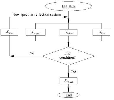
(3) Updating the specular reflection system: Once the coordinate of $X_{\rm New}$ is acquired, the eyes will change its place to continue searching for the "object", the four elements of the system are $X_0 X_1 X_2$ and $X_{\rm New}$ under the current situation. The specular reflection system will be adjusted by the modification of the four elements, the system will be changed by the rules shown in Fig. 1.
The optimization steps of the SRA are shown as follows:
Step 1: Define the initial value $X_i$ , $i = 0, 1, 2, 3$ , and the maximum iteration number $Iter_{\max}$ .
Step 2: If the precision or the maximum iteration number reaches the design requirements, the coordinate of $X_{\rm Object}$ will be output which is the optimum solution. Otherwise, execute the next step continually.
Step 3: Search the coordinate of $X_{\rm New}$ by (2) and (3), the new iteration process will begin, then go back to Step 2 and Continue to calculate.
In conclusion, the optimization flow chart of the SRA is given by Fig. 2.
2.3 Optimization Flow Chart of the SRA
Theorem 1: The constraint optimization problem presented in (1) can converge to the global extremum with 100 % probability by the SRA.
Proof: Provided that $X_{\rm Object} = \min f(X)$ , $X\in D$ which is the global optimal solution, where $f(X_{\rm Object})$ is the optimal value of objective function, $D$ is the feasible region and $D=\{X|g_j (X_{\rm Object}) = 0$ , $j = 1, 2, \ldots, m$ ; , $k$ $=$ $1$ , $2$ , $\ldots$ , $l$ ; and $D\in \mathbb{R}^N$ .
First, get the feasible initial solutions $X_{\rm Suspect}^0$ , $X_{\rm Mirror}^0$ and $X_{\rm Eyes}^0$ randomly among the searching space, where $X_{\rm Suspect}^0$ , $X_{\rm Mirror}^0$ , , and the corresponding values of objective function $f (X_{\rm Suspect}^0)$ , $f(X_{\rm Mirror}^0)$ and $f(X_{\rm Eyes}^0)$ can be worked out, where $f(X_{\rm Mirror}^0)$ $\leq$ $f(X_{\rm Eyes}^0)$ .
Second, the new solutions $f(X_{\rm Suspect}^k)$ , and $f(X_{\rm Eyes}^k)$ can be acquired according to the new specular reflection system, where are the randomly produced solutions which are uniformly distributed in , $X_{\rm Suspect}^k$ is the solution of the $k$ th ( iteration, $X_{\min}^k$ and $X_{\max}^k$ are the boundaries of design variable in the current iteration, and the maximum iteration number $Iter_{\max}$ should be big enough. Therefore, under the uniform distribution, the probability of generating the feasible solutions is:
$ \begin{align} p^k =&\ \int\nolimits_{X_{\rm Object} - \varepsilon }^{X_{\rm Object} + \varepsilon } \frac{1}{X_{\max }^k - X_{\min }^k }dX = \frac{2\varepsilon }{X_{\max }^k - X_{\min }^k } \nonumber\\[2mm] \ge&\ \frac{2\varepsilon }{X_{\max } - X_{\min } } > 0 \end{align} $
(4) where $\varepsilon$ is a real number which is sufficiently small; $X_{\rm max}$ and $X_{\rm min}$ are the extreme values of the 4 $\times N$ dimensional Euclidean space.
The probability that the feasible solution $X_{\rm Suspect}^0$ is optimal is $P^1$ , and the probability that $X_{\rm Suspect}^0$ is not optimal is $Q^1$ , both $P^1$ and $Q^1$ are expressed as follows:
$ \begin{align} \begin{cases} P^1 = P\{X_{\rm Suspect}^0 \subseteq [X_{\rm Object}-\varepsilon, X_{\rm Object} + \varepsilon]\} \\ \quad\quad\quad\quad\quad\quad\quad\quad\quad\mbox{ }P^1 = P \\ Q^1 = P\{X_{\rm Suspect}^0 \not\subset [X_{\rm Object}-\varepsilon, X_{\rm Object} + \varepsilon]\} \\ \quad\quad\quad\quad\quad\quad\quad\quad\quad\mbox{ }Q^1 = P \end{cases} \end{align} $
(5) where $X_{\rm Suspect}^0$ is the feasible solution gotten for the first time.
The probability that the feasible solution gotten for the second time still failing to be the optimal value is:
$ \begin{align} Q^2=Q^1(1-P)=(1-P)^2. \end{align} $
(6) So, the probability that the solution is optimal is:
$ \begin{align} P^2=1-(1-P)^2. \end{align} $
(7) After $n$ times iteration, the probability of getting the optimum solution can be acquired by the following inference.
$ \begin{align}\label{2} P^n& = 1 - (1 - P)^n = 1 - \prod _{i = 1}^n \left( {1 - \frac{2\varepsilon }{X_{\max }^i - X_{\min }^i }} \right) \nonumber\\[1mm] &\ge 1 - \left( {1 - \frac{2\varepsilon }{X_{\max } - X{ }_{\min }}} \right) ^n. \end{align} $
(8) Calculate the extreme value of (8):
$ \begin{align} \lim _{n \to \infty } P^n& = \lim\limits_{n \to \infty } \left[{1- \prod _{i = 1}^n \left( {1-\frac{2\varepsilon }{X_{\max }^i- X_{\min }^i }} \right)} \right] \nonumber\\ &\ge \lim _{n \to \infty } \left[{1-\left( {1- \frac{2\varepsilon }{X_{\max }-X_{\min } }} \right)^n} \right] = 1. \end{align} $
(9) With the iterations going on, it is more and more likely to achieve the optimum solution. When $n\rightarrow \infty$ , , it indicates that the searching process of SRA can converge to the global extreme with 100 % probability.
2.4 Selection of Control Parameter
The control parameter is closely related to the space complexity of optimized target, which has an effect on the capability of algorithm. The control parameters of classical optimization algorithm are gotten by experience or experiment, such as the learning parameter $c_1 = c_2$ = 2 by PSO [16], [17], and the crossover probability and mutation probability of GA [18]. It is impossible that the control parameter acquired by experience is suitable for all optimization problems. The SRA only has the control parameter $\xi$ , whose value will have a prominent effect on SRA. In this section, a classical test function is used to confirm the most appropriate value of $\xi$ , and the results are listed in Table Ⅰ.
表 Ⅰ JUDGEMENT OF $\xi$Table Ⅰ JUDGEMENT OF $\xi$Value of $\xi$ N =2 N =10 N=20 N=50 N = 100 Optimal solution (10-6) Iteration times Optimal solution (10-6) Iteration times Optimal solution (10-6) Optimal solution (103) Optimal solution (10-6) Optimal solution (103) Optimal solution (10-6) Optimal solution (104) 0.4 4.7776 402.70 7.1895 1103 7.2883 2.0369 8.9324 6.1015 9.5844 1.4945 0.5 3.3845 341.04 6.4267 940.12 7.3111 1.8001 8.4771 5.3149 9.6383 1.2586 0.6 3.9884 737.76 5.4844 936.46 7.2327 1.6802 9.0155 4.8292 9.3691 1.1344 0.7 3.5625 515.18 6.9587 810.24 7.2858 1.5971 8.5419 4.4544 9.5971 1.0679 0.8 4.2770 509.46 6.7379 747.90 7.5046 1.4992 8.8811 4.2697 9.3384 1.0741 0.9 4.0589 259.08 6.3850 732.90 7.4304 1.4562 8.3421 4.2036 9.4009 1.0976 1.0 4.9287 193.26 5.9257 694.18 6.8977 1.3677 8.3414 4.3603 9.5947 1.1404 1.1 4.6702 142.60 6.1496 674.28 8.0852 1.2946 9.4538 4.2854 9.4944 1.1889 1.2 4.6250 142.42 5.8875 626.54 7.7654 1.3608 8.6969 4.4775 9.6771 1.2434 1.3 5.1501 139.08 6.5208 654.72 7.2172 1.4050 8.9588 4.5342 9.5792 1.3215 1.4 5.4409 131.02 5.6072 695.40 6.9556 1.4699 8.9053 4.6930 9.6898 1.3675 1.5 4.7099 103.72 5.7050 675.02 7.6612 1.4740 9.0472 4.8329 9.5134 1.4173 1.6 4.7625 93.82 5.8038 713.20 6.4546 1470 8.9756 4.8634 9.7748 1.4768 1.7 4.9327 91.94 4.9871 783.90 5.8034 1.6036 9.1825 5.0851 9.6612 1.4985 1.8 5.9076 87.32 5.4104 856.30 7.1143 1.6917 8.7372 5.3202 9.4446 1.5536 1.9 4.9402 82.44 5.5724 832.12 6.4092 1.8641 8.7754 5.5962 9.6617 1.6423 2.0 4.7168 89.08 4.8307 998.300 5.7508 2.0544 8.1780 6.3700 9.4975 2.5117 $ \begin{align} f (x_1, x_2, \ldots, x_N)=\sum\limits_{j=1}^N j\times x_j^2. \end{align} $
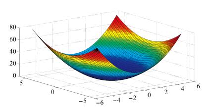
(10) The test function is illustrated by (10), and its three-dimension diagram is shown in Fig. 3. The global minimum value in theory of this function is 0 $(0, 0, \ldots, 0)$ and the constraint condition is $-5.12\leq x_j\leq 5.12$ , $j=1, 2, \ldots, N$ . In consideration of $N = (2, 10, 20, 50, 100, 500)$ and $\xi = (0.4$ , $0.5$ , $\ldots$ , $2.0)$ , do the calculation 50 times using every possible combination of $N$ and $\xi$ , then put the average results in Table Ⅰ. Assume that the convergence condition is $Iter_{\max}$ $=$ $10^5$ or $f (x_1, x_2, \ldots, x_N )\leq 10^{-5}$ .
As shown in Table Ⅰ, all the results fall in between 10 $^{-5}$ and 10 $^{-6}$ , the optimization efficiency which is influenced by $\xi$ cannot be evaluated by the optimal solutions, therefore, iteration times is the only factor to be considered.
According to the Table Ⅰ, the conclusions can be drawn as follows: when $N = 2$ and $\xi = 1.9$ , the efficiency of the optimization is highest, the corresponding iteration is 82.44; When $N = 10$ , , $N = 50$ and $N = 100$ , the best $\xi$ and its corresponding iteration times are 1.3 and 654.72, 1.1 and $1.2946\times 10^3$ , 0.9 and $4.2036\times 10^3$ , 0.7 and $1.0679$ $\times$ $10^4$ , respectively. In addition, the value of $\xi$ will be reduced gradually with the increasing of $N$ , and the relationship between $\xi$ and $N$ (as shown in (11)) can be speculated by the method of data fitting.
$ \begin{align} \xi=\frac{2.15}{N}+0.84. \end{align} $
(11) 2.5 Simulation Experiments
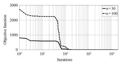
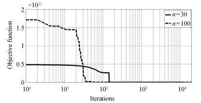
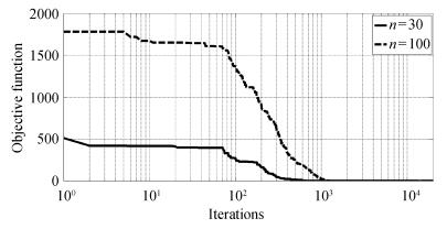
To verify the global optimization ability of SRA, four numerical test functions in [10] are used, each test function is listed in Table Ⅱ in detail. The total iteration time is set as 2000. The SRA will be executed 50 times, and the average values are listed in Table Ⅲ, other results are references from [10], Figs. 4-7 show the iteration curves of the objective functions of each test function respectively.
表 Ⅱ NUMERICAL CALCULATION FUNCTIONTable Ⅱ NUMERICAL CALCULATION FUNCTIONName Expression Interval of convergence Global extreme Dimension Sphere $f_1 = \sum\limits_{i = 1}^n {x_i^2 }$ $x_i\in [-50,50]$ 0 (0, 0, $\ldots$ , 0) $n$ = 30 100 Griewank $f_2 = 1 + \sum\limits_{i = 1}^n {\left( {\frac{x_i^2 }{4000}} \right) -\prod\limits_{i = 1}^n {\cos \left( {\frac{x_i }{\sqrt i }} \right)} }$ $x_i\in [-600,600]$ 0 (0, 0, $\ldots$ , 0) $n$ = 30 100 Rosenbrock $f_3 = \sum\limits_{i = 1}^{n - 1} {[100(x_{i + 1}-x_i^2 )^2 + (x_i-1)^2]}$ $x_i\in [-100,100]$ 0 (1, 1, $\ldots$ , 1) $n$ = 30 100 Restrigin $f_4 = \sum\limits_{i = 1}^n {[10 + x_i^2-10\cos (2\pi x_i )]}$ $x_i\in [-5.0, 5.0]$ 0 (0, 0, $\ldots$ , 0) $n$ = 30 100 表 Ⅲ CALCULATION RESULTS OF TEST FUNCTIONTable Ⅲ CALCULATION RESULTS OF TEST FUNCTIONName PSO
(n = 30) [10]Kalman swarm
(n = 30) [10]Chaos ant colony optimization
(n = 30)[10]Chaos PSO
(n = 30) [10]New chaos PSO
(n = 30) [10]SRA
(n = 30)SRA
(n = 100)Sphere 3.7004×10² 4.723 3.815×10⁻¹ 2.4736×10⁻³ 2.0729×10⁻⁹ 1.1080×10⁻²⁴ 2.3160×10⁻¹² Griewank 2.61×10⁷ 3.28×10³ 23.414 6.8481×10⁻² 9.9051×10⁻¹¹ 4.6629×10⁻¹⁵ 2.7978×10⁻¹⁴ Rosenbrock 13.865 9.96×10⁻¹ 4.669×10⁻¹ 1.0404×10⁻² 2.9068×10⁻⁴ 9.8730×10⁻⁷ 6.1173×10⁻⁵ Restrigin 1.0655×10² 53.293 22.6361 9.5258×10⁻¹ 4.3741×10⁻⁴ 3.9373×10⁻²¹ 8.7727×10⁻⁷ The results in Table Ⅳ indicate that: when $n$ = 30, the results of the four test functions calculated by SRA are , $4.6629 \times 10^{-15}$ , $9.8730 \times 10^{-7}$ and $3.9373$ $\times$ $10^{-21}$ respectively, which are , $2.12 \times 10 ^4$ , $2.90$ $\times$ $10^2$ , times higher than the results gotten by new chaos PSO algorithm which possesses the highest accuracy in [10]; When , the results of the four test functions calculated by SRA are $2.3160\times 10^{-12}$ , $2.7978$ $\times$ $10^{-14}$ , $6.1173\times10^{-5}$ , $8.7727\times 10^{-7}$ respectively, and the computational accuracy are still $8.95\times 10^2$ , , $4.75$ , $4.99$ $\times$ $10^2$ times higher than the results calculated by new chaos PSO algorithm. All in all, the SRA is an efficient optimization algorithm.
表 Ⅳ CALCULATION RESULTSTable Ⅳ CALCULATION RESULTSDesign method Design variables (mm) Objective function (mm2) Reliability Sensitivity of reliability/(10-3) x1 x2 x3 x4 x5 A Rv $\frac{\partial R_v}{\partial S}$ $\frac{\partial R_v}{\partial E}$ $\frac{\partial R_v}{\partial \rho}$ SRA Optimization 6 6 205 635 257 10 704 0.5071 14.3985 0.0017 9.15×10⁻⁹ 0.0011 Reliability Optimization 6 6 258 632 310 11 304 0.9968 13.0816 0.0015 8.77×10⁻⁹ 0.0010 Robust Reliability Optimization 6 6 324 595 376 11 652 0.9813 12.6270 0.0015 9.23×10⁻⁹ 0.0010 PSO Optimization 10 6 185 567 619 11 544 0.5314 13.0714 0.0015 9.8×10⁻⁹ 0.0010 Reliability Optimization 7 7 222 605 276 12 334 0.9806 12.9119 0.0015 9.73×10⁻⁹ 0.0011 Robust Reliability Optimization 9 6 302 534 354 12 780 0.9810 11.5262 0.0013 1.01×10⁻⁸ 0.0010 FOA Optimization 9 6 190 581 633 11 328 0.5132 13.3500 0.0016 9.64×10⁻⁹ 0.0010 Reliability Optimization 6 6 491 532 543 13 068 0.9802 11.3697 0.0013 1.01×10⁻⁸ 9.95×10⁻⁴ Robust Reliability Optimization 8 11 237 536 299 16 576 1.0 11.6479 0.0013 1.27×10⁻⁹ 0.0013 Note: The index of reliability R0 = 0.98 is deflned. 3. Reliability Robust Optimization Design
3.1 Reliability Design
According to the reliability design theory, the reliability can be calculated by (12):
$ \begin{align} R=\int_{g(X)} f_x(X) dX \end{align} $
(12) where $f_x (X)$ is the joint probability density of basic random variables $X=(X_1, X_2, \ldots, X_n)^T$ , which shows the state of the components.
$ \begin{align} \begin{cases} g(X)\leq 0, &{\rm failure}\\[2mm] g(X)>0, &{\rm safe.} \end{cases} \end{align} $
(13) The basic random variables $X_i$ ( $i = 1, 2, \ldots, n$ ) are independent of each other and follow certain distribution. The reliability index $\beta$ and the reliability $R=\Phi(\cdot)$ can be calculated by Monte Carlo method [19], where $\Phi(\cdot)$ is the standard normal distribution function.
3.2 Reliability Robust Optimization Design
Robust design is a modern design technique that can improve the efficiency and quality and reduce the cost of products [20], [21]. The robust design of mechanical products can make the products insensitive to the changes of design parameters. The product which is designed by robust design method has the characteristic of stability. Even if there is an error in the designed parameters, the product still has excellent performance. Reliability is a kind of design method to eliminate the weaknesses, failure modes and guard against malfunction. The reliability robust optimization design is a new method by combining the robust design and reliability design, which possess all the merits of the two methods. The products designed by the reliability robust optimization design method are reliable and have robustness.
$ \begin{align} &\min f(X)=\omega_1 f_1(X)+\omega_2 f_2(X)\notag\\ & {\rm s.t.} \ \ R\geq R_0\notag\\ &\qquad p_i(X)\geq 0, \ i=1, 2, \ldots, l\notag\\ &\qquad q_j(X)\geq 0, \ j=1, 2, \ldots, m \end{align} $
(14) where $f_1(X)$ and $f_2(X)$ are the objective functions of the Reliability Robust Optimization design, $f_1(X)=R$ and $f_2(X)$ is the design criterion related to robust design which can be acquired by (15); $R$ is the reliability; $R_0$ is the constraint condition of reliability; $p_i$ and $q_j$ are equality and inequality constraints of the robust reliability optimization design respectively.
$ \begin{align} f_2 (X) = \sqrt {\sum\limits_{i = 1}^n \left( {\frac{\partial R}{\partial X_i }} \right)^2} \end{align} $
(15) where $\omega_1$ and $\omega_2$ are weighting coefficients, which are related to the importance of $f_1(X)$ and $f_2(X)$ , both of them are calculated by (16), and $\omega_1+\omega_2 = 1$ .
$ \begin{align} \begin{cases} \omega _1 = \dfrac{f_2 (X^{1\ast }) - f_2 (X^{2\ast })}{[f_1 (X^{2\ast })- f_1 (X^{1\ast })] + [f_2 (X^{1\ast })-f_2 (X^{2\ast })]} \\[4mm] \omega _2 = \dfrac{f_1 (X^{2\ast }) - f_1 (X^{1\ast })}{[f_1 (X^{2\ast })- f_1 (X^{1\ast })] + [f_2 (X^{1\ast })-f_2 (X^{2\ast })]} \end{cases} \end{align} $
(16) where $X^{1*}$ and $X^{2*}$ are the best values when $\min f(X)$ $=$ $f_1 (X)$ and $\min f(X)=f_2 (X)$ respectively.
4. Engineering Example
The bridge crane is taken as an example to verify the capability of the SRA in solving the engineering problems. The SRA is adopted to design the structure with optimized design, reliability optimization design and robust reliability optimization design, and the results are listed in Table Ⅲ together with the results calculated by PSO and FOA, which are used for analysing the performance of the SRA.
4.1 Design Parameters
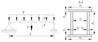
The mechanical model of the bridge crane is shown in Fig. 8, the uniform load $q$ and the concentrated load $F$ are exerted on the girder, where $q$ is caused by the structure deadweight and $F$ is related to the weight of the hoisted cargo.
The parameters $x_i$ $(i = 1, 2, 3, 4, 5)$ are considered to be the design variables, where $6\leq x_1$ , $x_2\leq 30$ , $50\leq x_3$ , $x_4$ $\leq$ $5000$ , $x_5 = x_3 + 2x_2 + 40$ . The parameter $S$ is the span of the bridge crane. Other parameters include the elasticity modulus $E$ , the material density $\rho$ , $q$ $=$ $g(x_1$ , $x_2$ , $x_3$ , $x_4, x_5)$ . The parameters $S$ , $F$ , $E$ and $\rho$ are independent of each other, and they are normal random variables, $S$ $\sim$ ${\rm N}(12, 0.08^2)$ , $F$ $\sim$ , $E$ $\sim$ ${\rm N}(206 000$ , $6180^2)$ , $\rho\sim {\rm N}(7850, 5.6^2)$ .
4.2 Optimization Design
Objective function: According to the characteristics of the structural optimization problem, the objective function can be defined as shown in (17).
$ \begin{align} {\rm min} f(x_1, x_2, x_3, x_4, x_5)=2x_1x_5+2x_2x_4. \end{align} $
(17) Constraint condition: Strength, stiffness and stability are the three basic failure modes of bridge crane. Therefore, the constraint condition can be defined as following:
1) Strength Constraint: The maximum stress of dangerous point in mid-span section must be smaller than the ultimate stress $f_{rd}$ ;
$ \begin{align} &h_1(x_1, x_2, x_3, x_4, x_5)=f_{rd}-\sigma\notag\\ &\qquad =f_{rd}-\frac{qS^2+2FS}{8I_Z}\left(\frac{x_4}{2}+x_1\right) \end{align} $
(18) where $f_{rd}$ is determined by the limit state method, and $f_{rd}$ $=$ ${f_{yk}}/{\gamma_m} = {235}/{1.1}=213.64$ MPa, $f_{(yk)}$ = 235 is yield stress, $\gamma_m$ = 1.1 is the resistance coefficient, $I_Z$ is moment of inertia of Section 2.1, $q$ and $I_Z$ are the functions related to design variables $x_i$ ( $i$ = 1, 2, 3, 4, 5).
2) Stiffness Constraint: The maximum deflection of the structure must be smaller than the allowable value $\gamma_0$ $=$ $S/400$ .
$ \begin{align} &h_2(x_1, x_2, x_3, x_4, x_5)=\gamma_0-\gamma\notag\\ &\qquad =\gamma_0-\left(\frac{5qS^4}{384EI_Z}+\frac{FS^3}{48EI_Z}\right). \end{align} $
(19) 3) Stability Constraint: The depth-width ratio of Section 2.1 must be smaller than 3.
$ \begin{align} h_3(x_1, x_2, x_3, x_4, x_5)=3-\frac{x_4+2x_1}{x_3+2x_2}. \end{align} $
(20) In conclusion, the optimization model of the bridge crane can be built as (21).
$ \begin{align} & \min f(x_1, x_2, x_3, x_4, x_5) \notag\\ & {\rm s.t.} \ \ h_k(x_1, x_2, x_3, x_4, x_5)\geq 0, \quad k=1, 2, 3\notag \\ &\qquad 6\leq x_1, \ x_2\leq 30\notag \\ &\qquad 50\leq x_3, \ x_4\leq 5000. \end{align} $
(21) 4.3 Reliability Optimization Design
The reliability constraint of structure is added to (21) to achieve the reliability optimization design. The failure of any mode will result in the failure of the structure, so the reliability $R_v$ is defined by (22). The reliability optimization model of bridge crane can be established by (23).
$ \begin{align} R_v=\prod\limits_{k=1}^3 R_k %(h_k\geq 0) \end{align} $
(22) where $R_k$ , $k=1, 2, 3$ is the probability of the $k$ th failure mode.
$ \begin{align} & \min f(x_1, x_2, x_3, x_4, x_5)\notag \\ & {\rm s.t.}\ \ h_k(x_1, x_2, x_3, x_4, x_5)\geq 0, \quad k=1, 2, 3\notag\\ &\qquad 6\leq x_1, \ x_2\leq 30\notag\\ &\qquad 50\leq x_3, \ x_4\leq 5000\notag\\ &\qquad R_v-R_0\geq 0. \end{align} $
(23) 4.4 Robust Reliability Optimization Design
According to the robust reliability optimization design model which is shown in (14), the index of reliability and robustness are taken into account, the multi-objective optimization model is built by (24).
$ \begin{align} & \min \omega_1\times f(x_1, x_2, x_3, x_4, x_5)+w_2\times f'(x)\notag \\ & {\rm s.t.} \ \ h_k(x_1, x_2, x_3, x_4, x_5)\geq 0, \quad k=1, 2, 3\notag\\ &\qquad 6\leq x_1, \ x_2\leq 30\notag\\ &\qquad 50\leq x_3, \ x_4\leq 5000\notag\\ &\qquad R_v-R_0\geq 0 \end{align} $
(24) where .
4.5 Calculation Results
The three optimization models shown in (21), (23) and (24) are calculated by the SRA, PSO and FOA, respectively. And the results are presented in Table Ⅲ, from which the conclusions can be drawn as follows:
1) For structural optimization, the results obtained by the three algorithms are 10 704, 11 544 and 11 328, the optimum among the three is 10 704 which is calculated by the SRA, which proves the ability of SRA is higher than PSO and FOA. The reliability results of the three groups of parameters are 0.5071, 0.5314 and 0.5132 respectively, which are unable to meet the requirement of reliability design for the reliability constraint is ignored.
2) The reliability of the structure can be ensured and the robustness can be improved after reliability optimization design. However, the areas of Section 2.1 are increased to 11 652, 12 334 and 16 576 at the same time, and the best result is also calculated by SRA.
3) With the requirements of the robustness, the reliability sensitivity index of design variables are significantly reduced, and the robustness of structure is improved notably.
5. Conclusions
In this paper, a new optimization algorithm — specular reflection algorithm (SRA) is proposed, which is inspired by the optical property of the mirror. The SRA has a particular searching strategy which is different from the swarm intelligence optimization algorithms. The convergence ability of the SRA is verified by the traditional mathematical method, it converges to the global optimum value with the probability of 100 %. The reasonable values of the control parameters are analysed, and their computational formula is deduced by the method of data fitting, so that the control parameters will vary with the different problems and thus the adaptation and the operability of the SRA will be improved. Four classical numerical test functions are analysed by the SRA, and the results indicate that the ability of the SRA is better than the traditional intelligent optimization algorithms. Then, the theories of the reliability optimization and robust design are combined to establish the mathematical models of the optimization design, reliability optimization design and robust reliability optimization design for the bridge crane as an example system, which are calculated by the SRA and other two optimization methods (PSO and FOA). The conclusions are drawn after the simulation, that the structure designed by the SRA is reliable and robust. The results calculated by the SRA are superior to the PSO and the FOA. All in all, the SRA is the latest research in the area of intelligent optimization, which has the better calculation capability than other optimization algorithms, and the ability for the structure design is verified in this paper. SRA can be widely applied in other fields and create more value.
-
-
[1] 武雷, 保宏, 杜敬利, 王从思. 一种自抗扰控制器参数的学习算法. 自动化学报, 2014, 40(3): 556-560 http://www.aas.net.cn/CN/abstract/abstract18321.shtmlWu Lei, Bao Hong, Du Jing-Li, Wang Cong-Si. A learning algorithm for parameters of automatic disturbances rejection controller. Acta Automatica Sinica, 2014, 40(3): 556-560 http://www.aas.net.cn/CN/abstract/abstract18321.shtml [2] 韩京清. 自抗扰控制技术—估计补偿不确定因素的控制技术. 北京: 国防工业出版社, 2008.Han Jing-Qing. Active Disturbance Rejection Control Technique—The Technique for Estimating and Compensating the Uncertainties. Beijing: National Defense Industry Press, 2008. [3] Han J Q. From PID to active disturbance rejection control. IEEE Transactions on Industrial Electronics, 2009, 56(3): 900-906 doi: 10.1109/TIE.2008.2011621 [4] Sira-Ramírez H, Linares-Flores J, García-Rodríguez C, Contreras-Ordaz M A. On the control of the permanent magnet synchronous motor: an active disturbance rejection control approach. IEEE Transactions on Control Systems Technology, 2014, 22(5): 2056-2063 doi: 10.1109/TCST.2014.2298238 [5] Yao J Y, Jiao Z X, Ma D M. Extended-state-observer-based output feedback nonlinear robust control of hydraulic systems with backstepping. IEEE Transactions on Industrial Electronics, 2014, 61(11): 6285-6293 doi: 10.1109/TIE.2014.2304912 [6] 马红雨, 苏剑波. 基于自抗扰控制器的机器人无标定三维手眼协调. 自动化学报, 2004, 30(3): 400-406 http://www.aas.net.cn/CN/abstract/abstract16332.shtmlMa Hong-Yu, Su Jian-Bo. Uncalibrated robotic 3D hand-eye coordination based on auto disturbance rejection controller. Acta Automatica Sinica, 2004, 30(3): 400-406 http://www.aas.net.cn/CN/abstract/abstract16332.shtml [7] Castañeda L A, Luviano-Juárez A, Chairez I. Robust trajectory tracking of a Delta robot through adaptive active disturbance rejection control. IEEE Transactions on Control Systems Technology, 2015, 23(4): 1387-1398 doi: 10.1109/TCST.2014.2367313 [8] Zhu Z, Xu D, Liu J M, Xia Y Q. Missile guidance law based on extended state observer. IEEE Transactions on Industrial Electronics, 2013, 60(12): 5882-5891 doi: 10.1109/TIE.2012.2232254 [9] 薛文超, 黄朝东, 黄一. 飞行制导控制一体化设计方法综述. 控制理论与应用, 2013, 30(12): 1511-1520 http://www.cnki.com.cn/Article/CJFDTOTAL-KZLY201312007.htmXue Wen-Chao, Huang Chao-Dong, Huang Yi. Design methods for the integrated guidance and control system. Control Theory and Applications, 2013, 30(12): 1511-1520 http://www.cnki.com.cn/Article/CJFDTOTAL-KZLY201312007.htm [10] 熊少锋, 王卫红, 刘晓东, 王森, 武亮. 考虑导弹自动驾驶仪动态特性的带攻击角度约束制导律. 控制与决策, 2015, 30(4): 585-592 http://youxian.cnki.com.cn/yxdetail.aspx?filename=KZYC20141205002&dbname=CAPJ2015Xiong Shao-Feng, Wang Wei-Hong, Liu Xiao-Dong, Wang Sen, Wu Liang. Impact angle guidance law considering missile's dynamics of autopilot. Control and Decision, 2015, 30(4): 585-592 http://youxian.cnki.com.cn/yxdetail.aspx?filename=KZYC20141205002&dbname=CAPJ2015 [11] 刘晓东, 黄万伟, 禹春梅. 含扩张状态观测器的高超声速飞行器动态面姿态控制. 宇航学报, 2015, 36(8): 916-922 http://www.cnki.com.cn/Article/CJFDTOTAL-YHXB201508008.htmLiu Xiao-Dong, Huang Wan-Wei, Yu Chun-Mei. Dynamic surface attitude control for hypersonic vehicle containing extended state observer. Journal of Astronautics, 2015, 36(8): 916-922 http://www.cnki.com.cn/Article/CJFDTOTAL-YHXB201508008.htm [12] 黄一, 张文革. 自抗扰控制器的发展. 控制理论与应用, 2002, 19(4): 485-492 http://www.cnki.com.cn/Article/CJFDTOTAL-KZLY200204000.htmHuang Yi, Zhang Wen-Ge. Development of active disturbance rejection controller. Control Theory and Applications, 2002, 19(4): 485-492 http://www.cnki.com.cn/Article/CJFDTOTAL-KZLY200204000.htm [13] 夏元清, 付梦印, 邓志红, 任雪梅. 滑模控制和自抗扰控制的研究进展. 控制理论与应用, 2013, 30(2): 137-147 http://www.cnki.com.cn/Article/CJFDTOTAL-KZLY201302000.htmXia Yuan-Qing, Fu Meng-Yin, Deng Zhi-Hong, Ren Xue-Mei. Recent developments in sliding mode control and active disturbance rejection control. Control Theory and Applications, 2013, 30(2): 137-147 http://www.cnki.com.cn/Article/CJFDTOTAL-KZLY201302000.htm [14] 高志强. 自抗扰控制思想探究. 控制理论与应用, 2013, 30(12): 1497-1509 http://www.cnki.com.cn/Article/CJFDTOTAL-KZLY201312006.htmGao Zhi-Qiang. On the foundation of active disturbance rejection control. Control Theory and Applications, 2013, 30(12): 1497-1509 http://www.cnki.com.cn/Article/CJFDTOTAL-KZLY201312006.htm [15] Zheng Q, Gao L Q, Gao Z Q. On stability analysis of active disturbance rejection control for nonlinear time-varying plants with unknown dynamics. In: Proceedings of the 46th IEEE Conference on Decision and Control. New Orleans, USA: IEEE, 2007. 3501-3506 [16] Guo B Z, Zhao Z L. On the convergence of an extended state observer for nonlinear systems with uncertainty. Systems and Control Letters, 2011, 60(6): 420-430 doi: 10.1016/j.sysconle.2011.03.008 [17] Zheng Q, Gao L Q, Gao Z Q. On validation of extended state observer through analysis and experimentation. Journal of Dynamic Systems, Measurement, and Control, 2012, 134(2): 024505, DOI: 10.1115/1.4005364 [18] 陈增强, 孙明玮, 杨瑞光. 线性自抗扰控制器的稳定性研究. 自动化学报, 2013, 39(5): 574-580 http://www.aas.net.cn/CN/abstract/abstract17868.shtmlChen Zeng-Qiang, Sun Ming-Wei, Yang Rui-Guang. On the stability of linear active disturbance rejection control. Acta Automatica Sinica, 2013, 39(5): 574-580 http://www.aas.net.cn/CN/abstract/abstract17868.shtml [19] 张洪华, 关轶峰, 胡锦昌, 王泽国. 分区四元数姿态控制. 自动化学报, 2015, 41(7): 1341-1349 http://www.aas.net.cn/CN/abstract/abstract18707.shtmlZhang Hong-Hua, Guan Yi-Feng, Hu Jin-Chang, Wang Ze-Guo. A novel attitude control strategy based on quaternion partition. Acta Automatica Sinica, 2015, 41(7): 1341-1349 http://www.aas.net.cn/CN/abstract/abstract18707.shtml [20] 杨明, 董晨, 王松艳, 晁涛. 基于有限时间输出反馈的线性扩张状态观测器. 自动化学报, 2015, 41(1): 59-66 http://www.aas.net.cn/CN/abstract/abstract18583.shtmlYang Ming, Dong Chen, Wang Song-Yan, Chao Tao. Linear extended state observer based on finite-time output feedback. Acta Automatica Sinica, 2015, 41(1): 59-66 http://www.aas.net.cn/CN/abstract/abstract18583.shtml 期刊类型引用(4)
1. 戚其松,徐航,董青,辛运胜. 基于镜面反射算法的机械产品结构稳健优化设计. 机械设计与制造. 2024(01): 318-326 .  百度学术
百度学术2. 马兵,吕彭民,韩红安,刘永刚,李瑶,胡永涛. 共享多镜面反射优化算法及其在机械优化设计中的应用. 机械设计. 2024(12): 129-138 .  百度学术
百度学术3. 肖浩,肖林,贺宾,赵章焰. 基于人工蜂鸟算法的门式起重机主梁安全优化设计. 机械设计与研究. 2023(03): 222-226+231 .  百度学术
百度学术4. 于燕南,戚其松,董青,徐格宁. 多工况下的桥式起重机有限元分析及优化设计. 科学技术与工程. 2021(31): 13334-13341 .  百度学术
百度学术其他类型引用(7)
-


 下载:
下载:


 下载:
下载:
