

-
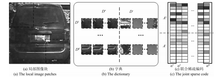
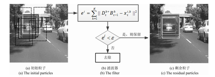
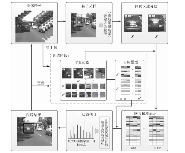
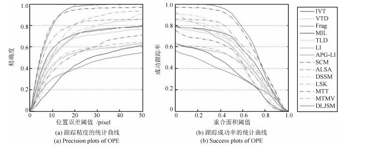
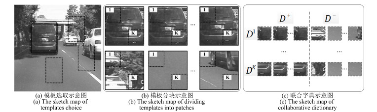
摘要: 目标表观建模是基于稀疏表示的跟踪方法的研究重点, 针对这一问题, 提出一种基于判别性局部联合稀疏表示的目标表观模型, 并在粒子滤波框架下提出一种基于该模型的多任务跟踪方法(Discriminative local joint sparse appearance model based multitask tracking method, DLJSM).该模型为目标区域内的局部图像分别构建具有判别性的字典, 从而将判别信息引入到局部稀疏模型中, 并对所有局部图像进行联合稀疏编码以增强结构性.在跟踪过程中, 首先对目标表观建立上述模型; 其次根据目标表观变化的连续性对采样粒子进行初始筛选以提高算法的效率; 然后求解剩余候选目标状态的联合稀疏编码, 并定义相似性函数衡量候选状态与目标模型之间的相似性; 最后根据最大后验概率估计目标当前的状态.此外, 为了避免模型频繁更新而引入累积误差, 本文采用每5帧判断一次的方法, 并在更新时保留首帧信息以减少模型漂移.实验测试结果表明DLJSM方法在目标表观发生巨大变化的情况下仍然能够稳定准确地跟踪目标, 与当前最流行的13种跟踪方法的对比结果验证了DLJSM方法的高效性.Abstract: Appearance modeling is the research focus in tracking method based on sparse representation. In this paper, a discriminative local joint sparse appearance model based multitask tracking method (DLJSM) is proposed within particle filter framework. The proposed model builds a discriminative dictionary for each image patch within the object-region in order to introduce the discriminative information into the local sparse model, and enhances the structure feature via joint sparse representation. During tracking, the target appearance is modeled firstly. Then the sampling particles are pre-selected according to the target appearance's consecutive changes characteristic to improve efficiency of the algorithm. Next, joint sparse representations of all the candidates are solved jointly. Furthermore, a function is defined to measure the similarities between candidates and the target model. Lastly, the target state is estimated by the maximum posterior probability. Besides, update is judged every five frames to avoid the accumulative error caused by frequent update and the target information in the first frame is reserved to alleviate drifting. Test results show that the proposed DLJSM tracker can maintain a stable and accurate tracking when the target appearance undergoes huge variations. Comparison results on challenging benchmark image sequences show that the DLJSM method out performs 13 other state-of-the-art algorithms.
-
Key words:
- Object tracking /
- appearance modeling /
- sparse representation /
- multitask tracking /
- particle filter
-
1. Introduction
Since recent few decades, some researchers focus their energy on the robust stability and controller design problems about the networked-control systems (NCSs) with some uncertain parameters because some networked-control systems have been succeeded in applications in modern complicated industry processes, e.g., aircraft and space shuttle, nuclear power stations, high-performance automobiles, etc. The fuzzy-logic control based on the Takagi-Sugeno (T-S) is widely used to dealing with complex nonlinear systems because it has simple dynamic structure and highly accurate approximation to any smooth nonlinear function in any compact set. One can consult [1]$-$[8] and the other cited literature therein [9]$-$[31]. Data-packet dropout is an important issue to be addressed in the networked-control systems [6], [32]. Zhang [33] solves the problem of $H_\infty$ estimation for a class of Markov jump linear systems but he neglect possible dropout in practice. Reference [34] reports the problem of $H_\infty$ stability of discrete-time switched linear system with average dwell time and with no dropout. In [6], piecewise Lyapunov function is proposed to analyze robust of the nonlinear NCSs without time-delay issue. Random data-packet dropout and time delay are well considered but the controlled NCSs are linear systems in [32]. Reference [8] discusses the problem of robust $H_\infty$ output feedback control for a class of continuous-time Takagi-Sugeno (T-S) fuzzy affine dynamic systems with parametric uncertainties and input constraints on ignoring some nonlinearities induced by system with data-packet dropout and random time delay. Reference [5] investigates the robust $H_\infty$ stability of a class of half nonlinear NCSs with multiple probabilistic delays and multiple missing measurements regardless of the dropout in the forward path. According to above consideration, we investigate a class of new nonlinear NCSs, in which not only sensors communicate with controllers by network but also controllers do with actuator in the same manner.
The highlights of this paper, which lie primarily on the new research problems and new system models, are summarized as follows:
1) A new model is established, in which the controllers communicate with the actuator by a wireless network and the random missing control from the controller to the actuator occurs and the sensors do with the controllers in the same manner.
2) The investigation on the T-S fuzzy model is used for a class of complex systems that describe the modeling errors, disturbance rejection attenuation, probabilistic delay, missing measurements and missing control within the same framework.
The rest of this paper is organized as follows. The problem under consideration is formulated in Section 2. Development of robust $H_{\infty}$ fuzzy control performance on the exponentially stability the closed-loop fuzzy system are placed in Section 3. Section 4 gives design of robust $H_\infty$ fuzzy controller. An illustrative example is given in Section 5, and we conclude the paper in Section 6.
Notation 1: The notation used in the paper is fairly standard. %The superscript "T" stands for matrix transpose; $\mathbb{R}^n$ denotes the $n$-dimensional real vectors; $\mathbb{R}^{m\times n}$ denotes the $n$-dimensional matrix; and $I$ and 0 represent the identity matrix and zero matrix, respectively. The notation $P>0$ ($P\geq 0$) means that $P$ is real symmetric and positive definite (semi-definite), ${\rm tr}(M)$ refers to the trace of the matrix $M$, and $ \|\cdot\|_2 $ stands for the usual $l_2$ norm. In symmetric block matrices or complex matrix expressions, we use an "$\star$" to represent a term that is induced by symmetry, and ${\rm diag}\{\cdots\}$ stands for a block-diagonal matrix. In addition, ${E}\{x\}$ and ${E}\{x|y\}$ will, respectively, mean expectation of $x$ and expectation of $x $ conditional on $y$.
2. Problem Formulation
In this note, the output feedback control problem for discrete-time fuzzy systems in NCSs is taken in our consideration, where the frame-work is depicted in Fig. 1.
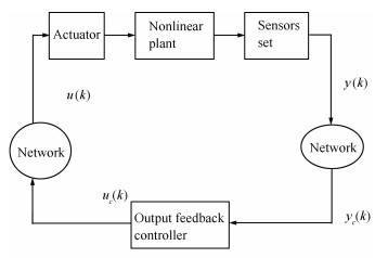 图 1 Framework of output feedback control systems over network environment.Fig. 1 Framework of output feedback control systems over network environment.
The sensors are connected to a network, which are shared by other NCSs and susceptible to communication delays and missing measurements or pack dropouts). As Fig. 1 depicts, pack dropouts from the controller to actuator can take place stochastically. The fuzzy systems with multiple stochastic communication delays and uncertain parameters can be read as follows:
Plant Rule $i$: If $\theta_{1}(k) $ is $ M_{i1}$, and $\theta_{2}(k)$ is $M_{i2}$, and, $\ldots$, and $\theta_{p}(k)$ is $M_{ip}$, then
$ \begin{align} x(k+1)=&\ A_i(k)x(k)+A_{di}\sum\limits_{m=1}^{h}\alpha_m(k)x(k-\tau_m(k))\notag\\ & +B_{1i}u(k)+D_{1i}v(k)\notag\\ \tilde{y}(k)=&\ C_ix(k)+D_{1i}v(k)\notag\\ z(k)=&\ C_{zi}(k)+B_{2i}u(k)+D_{3i}v(k)\notag\\ x(k)=&\ \phi(k)\quad\forall\, {k}\in \mathbb{Z}^{-}, ~\, i=1, \ldots, r \end{align} $
(1) where $M_{ij}$ is the fuzzy set, $r$ stands for the number of If-then rules, and $\theta(k)=[\theta_1(k), \theta_2(k), \ldots, \theta_{p}(k)]$ is the premise variable vector, which is independent of the input variable $u(k)$. $x(k)\in \mathbb{R}^n$ is the state vector, $u(k)\in \mathbb{R}^m$, $\tilde{y}$ $\in$ $\mathbb{R}^s$ is the process output, $z(k)\in \mathbb{R}^q$ is the controlled output, $v(k)\in \mathbb{R}^p$ presents a vector of exogenous inputs, which belongs to $l_2[0, \infty)$, $\tau_m(k)$ $(m=1, 2, \ldots, h)$ are the communication delays that vary with the stochastic variables $\alpha_m(k)$, and $\phi(k)$ $(\forall\, {k}\in \mathbb{Z}^{-})$ is the initial state.
The stochastic variables $\alpha_m(k)\in \mathbb{R}$ $(m=1, 2, \ldots, h)$ in (1) are assumed to satisfy mutually uncorrelated Bernoulli-distributed-white sequences described as follows:
$ \begin{align} & {\rm Prob}\{\alpha_m(k)=1\}={E}\{\alpha_m(k)\}=\bar{\alpha}_m\notag\\ & {\rm Prob}\{\alpha_m(k)=0\}=1-\bar{\alpha}_m.\notag \end{align} $
In this note, one can make the random communication-time delays satisfy the following assumption that the time-varying $\tau_m(k)$ $ (m=1, 2, \ldots, h)$ are subject to $ d_t\leq \tau_m(k)$ $\leq$ $d_T$. The matrices $A_i(k)=A_i+\Delta{A_i(k)}$, $C_{zi}(k)= C_{zi}$ $+$ $\Delta{C_{zi}}(k)$, where $ A_i, A_{di}, B_{1i}, B_{2i}, C_i, C_{zi}, D_{1i}, D_{2i}$, and $D_{3i}$ are known constant matrices with compatible dimensions. $\Delta{A_i(k)} $ and $\Delta C_{zi}(k)$ with the time-varying norm-bounded uncertainties satisfy
$ \begin{align} \left[ \begin{array}{c} \Delta A_i(k)\\ \Delta C_{zi}(k)\\ \end{array} \right]=\left[ \begin{array}{c} H_{ai}\\ H_{ci}\\ \end{array} \right]F(k)E \end{align} $
(2) with $H_{ai}$, $H_{ci}$ being constant matrices and $F^T(k)F(k)\leq I$, $\forall\, {k}$.
In this note, the packet dropout (the miss-measurement) read as
$ \begin{align} y_c(k)&= \Xi{C_i}x(k)+D_{2i}(k)\notag\\ &=\sum\limits_{l=1}^{s}\beta_lC_{il}x(k)+D_{2i}v(k)\notag\\ u(k)&=W(k)u_c(k)=W(k)C_{ki}x_c(k) \end{align} $
(3) where $\Xi=\hbox{diag}\{\beta_1, \ldots, \beta_s\}$ with $\beta_l$ $(l=1, 2, \ldots, s)$ being $s$ unrelated random variables, which are also unrelated with $\alpha_m(k)$ and $W(k)$ denoting the random packet missing from the controllers to the actuator. One can assume that $\beta_l $ has the probabilistic-density function $q_l(s)$ $(l=1, 2, \ldots, s)$ on the interval $[0, 1]$ with mathematical expectation $\mu_l$ and variance $\sigma_l^2$. $C_{il}={\rm diag}\{\underbrace{0, \ldots, 0}\limits_{l-1}, 1, \underbrace{0, \ldots, 0}\limits_{s-l}\}C_i$. We denote the stochastic pack dropouts from the controller to the actuator by $W(k)= {\rm diag}\{\omega_1(k), \ldots, \omega_m(k)\}$, where $\omega_l$ $(l=$ $1, 2, \ldots, m)$ are mutually unrelated random variables and obey Bernoulli distribution with mathematical expectation $\bar{\omega}_l$ and variance$\rho_l $and assumed to be unrelated with $\alpha_m(k)$. For a given pair of $(x(k), u(k))$, the final output of the fuzzy system is read as
$ \begin{align} x(k+1)=&\, \sum\limits_{i=1}^{r}h_i(\theta(k))[A_i(k)x(k)+B_{1, i}u(k)\notag\\ &\, +A_{di}\sum\limits_{m=1}^{h}x(k-\tau_m(k))+D_{1i}v(k)]\notag\\ y_c(k)=&\, \sum\limits_{i=1}^{r}h_i(\theta(k))[\Xi{C_i}x(k)+D_{2i}v(k)]\notag\\ z(k)=&\, \sum\limits_{i=1}^{r}h_i(\theta(k))[C_{zi}(k)x(k)+B_{2i}u(k)+D_{3i}v(k)] \end{align} $
(4) where the fuzzy-basis functions are described as
$ \begin{align} &{h_i(\theta(k))}=\frac {\vartheta_i(\theta(k))} {\sum\limits_{i=1}^{r}\vartheta_i(\theta(k))}\notag\\ &\vartheta_i(\theta(k))=\prod\limits_{j=1}^{p}M_{ij}(\theta_j(k))\notag \end{align} $
with $M_{ij}(\theta_j(k))$ being the grade of membership of $\theta_j(k)$ in $M_{ij}$. It is clear that $\vartheta_i(\theta(k))\geq 0$, $i=1, 2, \ldots, r$, $\sum_{i=1}^{r}\vartheta_i(\theta(k))>0$, $\forall\, {k}$, and $h_i(\theta(k))\geq 0$, $i=1, 2, \ldots, r$, $\sum_{i=1}^{r}h_i(\theta(k))=1$, $\forall\, {k}$. In the sequel, we denote $h_i=h_i(\theta(k))$ for brevity.
In the note, the fuzzy dynamic output-feedback controller for the fuzzy system (4) is given as
Controller Rule $i$: If $\theta_1(k)$ is $M_{il}$ and $\theta_2(k)$ is $M_{i2}$ and, $\ldots$, and $\theta_p(k)$ is $M_{ip}$ then
$ \begin{align} \begin{cases} x_c(k+1)=A_{ki}x_c(k)+B_{ki}y_c(k)\\ u(k)= W(k)C_{ki}x_c(k) \end{cases} \end{align} $
(5) with $x_c(k)\in \mathbb{R}^n$ being the controller state along with the controller parameters $A_{ki}$, $B_{ki}$ and $C_{ki}$ to be determined. Naturally, the overall fuzzy output-feedback controller is read as
$ \begin{align} \begin{cases} x_c(k+1)=\sum\limits_{i=1}^{r}h_i[A_{ki}x_c(k)+B_{ki}y(k)]\\ u(k)=\sum\limits_{i=1}^{r}h_iW(k)C_{ki}x_c(k), \ \ i=1, 2, \ldots, r. \end{cases} \end{align} $
(6) Combining (6) with (4), we can obtain the closed-loop system described as
$ \begin{align} \begin{cases} \bar{x}(k+1)=\sum\limits_{i-1}^{r}\sum\limits_{j=1}^{r}h_ih_j[(A_{ij}+B_{ij})\bar{x}(k)+D_{ij}v(k) \\ \qquad \qquad \quad\, +\sum\limits_{m=1}^{h}(\bar{A}_{dmi}+\tilde{A}_{dmi})\bar{x}(k-\tau_m(k)]\\ z(k)=\sum\limits_{i=1}^{r}\sum\limits_{j=1}^{r}h_ih_j[\bar{C}_{ij}(k)+\bar{\bar{C}}_{ij}]\bar{x}(k) +D_{3i}v(k) \end{cases} \end{align} $
(7) where
$ \begin{align*} &\bar{x}(k)=\left[ \begin{array}{c} x(k) \\ x_c(k) \\ \end{array} \right], \quad A_{ij}=\left[ \begin{array}{cc} A_i(k)&B_{1i}\bar{W}C_{kj} \\ B_{ki}\bar{\Xi}C_j&A_{ki} \\ \end{array} \right]\\[1mm] &B_{ij}=\left[ \begin{array}{cc} 0& B_{1i}\tilde{W}(k)C_{kj}\\ B_{ki}\tilde{\Xi}C_j& 0\\ \end{array} \right]\\[1mm] &\bar{A}_{dmi}=\left[ \begin{array}{cc} \bar{\alpha}_mA_{di}&0 \\ 0&0 \\ \end{array} \right], \quad \tilde{A}_{dmi}=\left[ \begin{array}{cc} \tilde{\alpha}_mA_{di}&0 \\ 0&0 \\ \end{array} \right]\\[1mm] &D_{ij}=\left[ \begin{array}{c} D_{1i} \\ B_{ki}D_{2j} \\ \end{array} \right], \quad \bar{C}_{ij}(k)=\bigg[ \begin{array}{cc} C_{zi}(k)&B_{2i}\bar{W}C_{kj} \\ \end{array} \bigg]\\[1mm] &\bar{\bar{C}}_{ij}(k)=\bigg[ \begin{array}{cc} 0&B_{2i}\tilde{W}(k)C_{kj} \\ \end{array} \bigg] \end{align*} $
with $\tilde{\alpha}_m(k)=\alpha_m(k)-\bar{\alpha}_m(k)$ and $\tilde{\omega}_j(k)={\omega}_j(k)-\bar{\omega}_j(k)$. It is evident that $E\{\tilde{\alpha}_m(k)\}=0$ and that $E\{\tilde{\omega}_j(k)\}=0$ and that $E\{\tilde{\alpha}_m^2(k)\}=\bar{\alpha}_m(1-\bar{\alpha}_m)=\sigma_m^2$ and that $E\{\tilde{\omega}_j^2(k)\}$ $=$ $\bar{\omega}_j(1-\bar{\omega}_j)=\rho_j^2$.
Denote
$ \begin{align*} &\bar{x}(k-\tau)\\ &=\left[ \!\!\begin{array}{cccc} \ \ \bar{x}^T(k-\tau_1(k)) &\!\bar{x}^T(k-\tau_2(k))&\! \cdots &\!\bar{x}^T(k-\tau_h(k))\ \ \\ \end{array} \!\!\right]^T\\ &\xi(k)=\left[ \begin{array}{ccc} \bar{x}^T(k)&\bar{x}^T(k-\tau) &v^T(k) \\ \end{array} \right]^T\end{align*} $
then (7) can also be rewritten as
$ \begin{align} \begin{cases} \bar{x}(k+1) =\sum\limits_{i=1}^{r}\sum\limits_{j=1}^{r}h_ih_j\left[A_{ij}\!+B_{ij}, \hat{Z}_{mi}\!+\Delta\hat{Z}_{mi}, D_{ij}\right]\xi(k) \\ z(k)=\sum\limits_{i=1}^{r}\sum\limits_{j=1}^{r}h_ih_j\left[\bar{C}_{ij}+ \bar{\bar{C}}_{ij}, 0, D_{3i}\right]\xi(k) \end{cases} \end{align} $
(8) where $\hat{Z}_{mi}=[\bar{A}_{d1i}, \ldots, \bar{A}_{dhi}]$ and $\Delta\hat{Z}_{mi}=[\tilde{A}_{d1i}, \ldots, \tilde{A}_{dhi}]$. In order to smoothly formulate the problem in the note, we introduce the following definition.
Definition 1: For the system (7) and every initial conditions $\phi$, the trivial solution is said to be exponentially mean square stable if, in the case of $v(k)=0$, there exist constants $\delta>0$ and $0<\kappa<1$ such that $E\{\|\bar{x}(k)\|^2\}$ $\leq$ $\delta\kappa^k \sup_{-d_M\leq i\leq 0}E\{\|{\phi(i)}\|^2\}$, $\forall\, {k}\geq 0$.
We will develop techniques to settle the robust $H_{\infty}$ dynamic output feedback problem for the discrete-time fuzzy system (7) subject to the following conditions:
1) The fuzzy system (7) is exponentially stable in the mean square.
2) Under zero-initial condition, the controlled output $z(k)$ satisfies
$ \begin{align} \sum\limits_{k=0}^{\infty}E\left\{\|{z(k)}\|^2\right\}\leq \gamma^2\sum\limits_{k=0}^{\infty}E\left\{\|{v(k)}\|^2\right\} \end{align} $
(9) for all nonzero $v(k)$, where $\gamma>0$ is a prescribed scalar.
Remark 1: The proposed new model has the function that not only the controllers communicate with the actuator by wireless but also the sensors do with the controllers by the same manner.
3. Development of Robust ${\pmb H}_{\pmb \infty}$ Fuzzy Control Performance
At first, we give the following lemma, which will be adopted in obtaining our main results.
Lemma 1 (Schur complement): Given constant matrices $S_1$, $S_2$, $S_3$, where $S_1=S_1^T$ and $0<S_2=S_2^T$, then $ S_1$ $+$ $S_3^TS_2^{-1}S_3$ $<$ $0$ if and only if
$ \begin{align*} \left[ \begin{array}{cc} S_1&S_3^T \\ S_3 &-S_2 \\ \end{array} \right]<0~~ \hbox{or}~~ \left[ \begin{array}{cc} -S_2&S_3 \\ S_3^T&S_1 \\ \end{array} \right]<0. \end{align*} $
Lemma 2 (S-procedure) [5]: Letting $L=L^T$ and $H$ and $E$ be real matrices of appropriate dimensions with $F$ satisfying $FF^T\leq I$, then $ L+HFE+E^TF^TH^T<0$ if and only if there exists a positive scalar $\varepsilon>0$ such that $L$ $+$ $\varepsilon^{-1}HH^T+\varepsilon E^TE<0$, or equivalently
$ \begin{align*} \left[ \begin{array}{ccc} L&H&\varepsilon{E^T} \\ H^T &-\varepsilon{I}&0 \\ \varepsilon{E}&0 &-\varepsilon{I} \\ \end{array} \right]<0. \end{align*} $
Lemma 3: For any real matrices $X_{ij}$ for $i$, $j=1, 2, \ldots, $ $r$ and $n>0$ with appropriate dimensions, we have [35]
$ \sum\limits_{i=1}^r\sum\limits_{j=1}^r\sum\limits_{l=1}^r\sum\limits_{l=1}^rh_ih_jh_kh_lX_{ij}^T\Lambda{X_{kl}}\leq\sum\limits_{i=1}^r\sum\limits_{j=1}^rh_ih_jX_{ij}^T\Lambda X_{ij}. $
Theorem 1: For given controller parameters and a prescribed $H_{\infty}$ performance $\gamma>0$, the nominal fuzzy system (7) is exponentially stable if there exist matrices $P>0$ and $Q_k$ $>$ $0$, $k=1, 2, \ldots, h$, satisfying
$ \left[ \begin{array}{cc} \Pi_i&\star \\ 0.5\Sigma_{ii}&\bigwedge \\ \end{array} \right]<0 $
(10) $ \left[ \begin{array}{cc} 4\Pi_i&\star \\ \Sigma_{ij}&\bigwedge \\ \end{array} \right]<0, \quad 1\leq i<j\leq r $
(11) where
$ \Pi_i =\ {\rm diag}\bigg\{-P+\sum\limits_{k=1}^h(d_T-d_t+1)Q_k, \hat{\alpha}\breve{A}_{di}^T\breve{P} \breve{A}_{di}\notag\\ \ \ \ \ \ \ -{\rm diag}\{Q_1, Q_2, \ldots, Q_h\}, -\gamma^2I\bigg\} $
(12) $\begin{align*} \hat{\alpha}=&\ {\rm diag}\left\{\bar{\alpha}_1(1-\bar{\alpha}_1), \ldots, \bar{\alpha}_h(1-\bar{\alpha}_h)\right\}\notag\\ \breve{A}_{di}=&\ {\rm diag}\{\underbrace{\hat{A}_{di}, \ldots, \hat{A}_{di}}\limits_h\}\notag\\ \check{C}_{ij}=&\ \left[\sigma_1\hat{C}_{11ij}^TP, \ldots\!, \sigma_s\hat{C}_{1sij}^TP, \rho_1\hat{C}_{k1ij}^TP, \ldots\!, \rho_m\hat{C}_{kmij}^TP\right]^T\notag\\ &\check{P}=\hbox{diag}\{\underbrace{P, \ldots, P}\limits_{s+m}\}\\ &{\small\bigwedge}=\hbox{diag}\{-\check{P}, -P, -I, \hbox{diag}\{\underbrace{-I, \ldots, -I}\limits_m\}\}\\ &\breve{P}=\hbox{diag}\{\underbrace{P, \ldots, P}\limits_h\}\\ &\hat{A}_{di}=\left[ \begin{array}{cc} A_{di}&0\\ 0&0\\ \end{array} \right] \\ &\Sigma_{ij}=\\ &\!\!\!\left[\!\!{\small \begin{array}{ccccc} \check{C}_{ij}\!+\!\check{C}_{ji}\! &\! 0\!&\!0 \\[2mm] PA_{ij}\!+\!PA_{ji} \! &\! P\hat{Z}_{mi}\!+\!P\hat{Z}_{mj} \! &\!PD_{ij}\!+\!PD_{ji}\\[2mm] \bar{C}_{ij}\!+\!\bar{C}_{ji}\! &\!0\! &\!D_{3i}\!+\!D_{3j}\\[2mm] \, [0 ~~ \rho_1B_{2i}C_{kj1}\!+\!\rho_1B_{2j}C_{ki1}] \! &\!0\! &\!0\\[2mm] \vdots\! &\!\vdots\! &\!\vdots\\[2mm] \, [0 ~~ \rho_mB_{2i}C_{kjm}\!+\!\rho_mB_{2j}C_{kim}]\! &\!0\! &\!0\\ \end{array}}\!\!\!\! \right]. \end{align*} $
Proof:
Let
$ \begin{align*} &\Theta_j(k)=\{x(k-\tau_j(k), x(k-\tau_j(k)+1, \ldots, x(k)\}\\ &\chi(k)=\{\Theta_1(k)\bigcup\Theta_2(k)\bigcup\ldots\bigcup\Theta_h(k)\}=\bigcup\limits_{j=1}^{h}\Theta_j(k) \end{align*} $
where $j=1, 2, \ldots, h$. We consider the following Lyapunov functional for the system of (7): $V(\chi(k))=\sum_{i=1}^3V_i(k)$, where
$ \begin{align*} &V_1(k)=\bar{x}^T(k)P\bar{x}\\ &V_2(k)=\sum\limits_{j=1}^{h}\sum\limits_{i=k-\tau_j(k)}^{k-1}\bar{x}^T(i)Q_j\bar{x}(i)\\ &V_3(k)=\sum\limits_{j=1}^h\sum\limits_{m=-d_M+1}^{-d_m}\sum\limits_{i=k+m}^{k-1}\bar{x}^T(i)Q_j\bar{x}(i) \end{align*} $
with $P>0$, $Q_j>0$ $(j=1, 2, \ldots, h)$ being matrices to be determined.
$ \begin{align} {E}[\Delta{V}|x(k)]&={E}[V(\chi(k+1))|\chi(k)]-V(\chi(k))\notag\\ & ={E}[(V(\chi(k+1))-V(\chi(k)))|\chi(k)]\notag\\ & =\sum\limits_{i=1}^{3}{E}[\Delta{V_i}|\chi(k)]. \end{align} $
(13) According to (7), we have
$ \begin{align*} &{E}\{\Delta{V_1}|\chi(k)\}\\ &\qquad={E} \left[(\bar{x}^T(k+1)P\bar{x}(k+1)-\bar{x}^T(k)P\bar{x}(k))|\chi(k)\right]\\ &\qquad\leq\xi^T(k)\sum\limits_{i=1}^{r}\sum\limits_{j=1}^{r}\Omega_{ij}\xi(k) \end{align*} $
where
$ \begin{align} & {{\Omega }_{ij}}=E\left\{ \left[\begin{matrix} A_{ij}^{T}P{{A}_{ij}}+B_{ij}^{T}P{{B}_{ij}}-P & {} \\ \star & {} \\ \star & {} \\ \end{matrix} \right. \right. \\ & \left. \left. \begin{matrix} {} & A_{ij}^{T}P{{{\hat{Z}}}_{mi}} & A_{ij}^{T}P{{D}_{ij}} \\ {} & \hat{Z}_{mi}^{T}P{{{\hat{Z}}}_{mi}}+\Delta \hat{Z}_{mi}^{T}P\Delta {{{\hat{Z}}}_{mi}} & \hat{Z}_{mi}^{T}P{{D}_{ij}} \\ {} & \star & D_{ij}^{T}P{{D}_{ij}} \\ \end{matrix} \right] \right\} \\ \end{align} $
$ {{B}_{ij}}=\left[\begin{matrix} 0 & 0 \\ {{B}_{ki}}\tilde{\Xi }{{C}_{j}} & 0 \\ \end{matrix} \right]+\left[\begin{matrix} 0 & {{B}_{1i}}\tilde{\omega }(k){{C}_{kj}} \\ 0 & 0 \\ \end{matrix} \right] $
$ \begin{align} & E\{B_{ij}^{T}P{{B}_{ij}}\} \\ & \ \ \ \ \ =\sum\limits_{l=1}^{s}{\sigma _{l}^{2}}{{\left[\begin{matrix} 0 & 0 \\ {{B}_{ki}}{{C}_{jl}} & 0 \\ \end{matrix} \right]}^{T}}P\left[\begin{matrix} 0 & 0 \\ {{B}_{ki}}{{C}_{jl}} & 0 \\ \end{matrix} \right] \\ & \ \ \ \ \ +\sum\limits_{l=1}^{m}{\rho _{l}^{2}}{{\left[\begin{matrix} 0 & {{B}_{1i}}{{C}_{kjl}} \\ 0 & 0 \\ \end{matrix} \right]}^{T}}P\left[\begin{matrix} 0 & {{B}_{1i}}{{C}_{kjl}} \\ 0 & 0 \\ \end{matrix} \right] \\ & \ \ \ ={{({{{\overset{\lower0.5em\hbox{$\smash{\scriptscriptstyle\smile}$}}{P}}}^{-1}}{{{\overset{\lower0.5em\hbox{$\smash{\scriptscriptstyle\smile}$}}{C}}}_{lij}})}^{T}}\overset{\lower0.5em\hbox{$\smash{\scriptscriptstyle\smile}$}}{P}({{{\overset{\lower0.5em\hbox{$\smash{\scriptscriptstyle\smile}$}}{P}}}^{-1}}{{{\overset{\lower0.5em\hbox{$\smash{\scriptscriptstyle\smile}$}}{C}}}_{lij}}) \\ \end{align} $
$ \begin{align} & \overset{\lower0.5em\hbox{$\smash{\scriptscriptstyle\smile}$}}{P}=\rm{diag}\{\underbrace{\mathit{P}, \ldots, \mathit{P}}_{\mathit{s}+\mathit{m}}\} \\ & {{{\hat{C}}}_{1lij}}=\left[\begin{matrix} 0 & 0 \\ {{B}_{ki}}{{C}_{jl}} & 0 \\ \end{matrix} \right] \\ & {{{\hat{C}}}_{klij}}=\left[\begin{matrix} 0 & {{B}_{1i}}{{C}_{kjl}} \\ 0 & 0 \\ \end{matrix} \right] \\ & {{{\overset{\lower0.5em\hbox{$\smash{\scriptscriptstyle\smile}$}}{C}}}_{ij}}={{\left[{{\sigma }_{1}}\hat{C}_{11ij}^{T}P, \ldots, {{\sigma }_{s}}\hat{C}_{1sij}^{T}P, {{\rho }_{1}}\hat{C}_{k1ij}^{T}P, \ldots, {{\rho }_{m}}\hat{C}_{kmij}^{T}P \right]}^{T}} \\ \end{align} $
$ \begin{align} & E\left\{ \Delta \hat{Z}_{mi}^{T}P\Delta {{{\hat{Z}}}_{mi}} \right\} \\ & \ \ \ \ \ =\sum\limits_{m=1}^{h}{{{{\bar{\alpha }}}_{m}}}(1-{{{\bar{\alpha }}}_{m}}){{\left[ \begin{matrix} {{A}_{di}} & 0 \\ 0 & 0 \\ \end{matrix} \right]}^{T}}P\left[ \begin{matrix} {{A}_{di}} & 0 \\ 0 & 0 \\ \end{matrix} \right] \\ & \ \ \ \ \ \ =\sum\limits_{m=1}^{h}{\hat{A}_{di}^{T}}P{{{\hat{A}}}_{di}}=\hat{\alpha }\overset{\lower0.5em\hbox{$\smash{\scriptscriptstyle\smile}$}}{A}_{di}^{T}\overset{\lower0.5em\hbox{$\smash{\scriptscriptstyle\smile}$}}{P}{{{\overset{\lower0.5em\hbox{$\smash{\scriptscriptstyle\smile}$}}{A}}}_{di}} \\ \end{align} $
$ \begin{align} & \hat{\alpha }=\rm{diag}\{{{{\bar{\alpha }}}_{1}}(1-{{{\bar{\alpha }}}_{1}}), \ldots, {{{\bar{\alpha }}}_\mathit{h}}(1-{{{\bar{\alpha }}}_\mathit{h}})\} \\ & {{{\overset{\lower0.5em\hbox{$\smash{\scriptscriptstyle\smile}$}}{A}}}_{di}}=\rm{diag}\{\underbrace{\mathit{{{\hat{A}}}_{di}}, \ldots, \mathit{{{\hat{A}}}_{di}}}_\mathit{h}\} \\ & E\{\Delta {{V}_{2}}|\chi (k)\}\le E\{\sum\limits_{j=1}^{h}{({{{\bar{x}}}^{T}}(}k){{Q}_{j}}\bar{x}(k) \\ & \ \ \ \ \ -{{{\bar{x}}}^{T}}(k-{{\tau }_{j}}(k)){{Q}_{j}}\bar{x}(k-{{\tau }_{j}}(k)) \\ & \ \ \ \ \ +\sum\limits_{i=k-{{d}_{M}}+1}^{k-{{d}_{m}}}{{{{\bar{x}}}^{T}}}(i){{Q}_{j}}\bar{x}(i))|\chi (k)\} \\ & E\{\Delta {{V}_{3}}|\chi (k)\}=E\{\sum\limits_{j=1}^{h}{((}{{d}_{T}}-{{d}_{t}}){{{\bar{x}}}^{T}}(k){{Q}_{j}}\bar{x}(k) \\ & \ \ \ \ \ -\sum\limits_{i=k-{{d}_{m}}+1}^{k-{{d}_{m}}}{{{{\bar{x}}}^{T}}}(i){{Q}_{j}}\bar{x}(i))|\chi (k)\}. \\ \end{align} $
It is clear that
$ {E}\{\Delta{V_2}|\chi(k)\}+{E}\{\Delta{V_3}|\chi(k)\}\leq\xi^T(k)T_{ij}\xi(k) $
with
$ \begin{align*} T_{ij}=&\ \hbox{diag}\Bigg\{\sum\limits_{k=1}^h(d_T-d_t+1)Q_k, \\ &-\hbox{diag}\{Q_1, Q_2, \ldots, Q_h\}, 0\Bigg\}.\end{align*} $
Therefore, we have ${E}\{\Delta{V}|\chi(k)\}\leq\xi^T(k)\Gamma_{ij}\xi(k)$, where $\Gamma_{ij}$ $=$ $\Omega_{ij}+T_{ij}$. Due to
$ \begin{align*} &{E}\left\{z^T(k)z(k)-\gamma^2v^T(k)v(k)\right\}\\ &\qquad\leq\xi(k)\sum\limits_{i=1}^r\sum\limits_{j=1}^rh_ih_j {E}\left\{[\bar{C}_{ij}+\bar{\bar{C}}_{ij}, 0, D_{3i}]^T\right.\\ &\qquad\quad \left.\times[\bar{C}_{ij}+\bar{\bar{C}}_{ij}, 0, D_{3i}] - \hbox{diag}\{0, 0, \gamma^2I\}\right\}\xi(k) \end{align*} $
we can obtain
$ \begin{align*} &{E}\left\{z^T(k)z(k)-\gamma^2v^T(k)v(k)+\Delta{V(k)}\right\}\\ &\qquad \leq\xi^T(k)({\Omega}_{ij}^T\hbox{diag} \{P, I\}{\Omega}_{ij}\\ &\qquad\quad +\mathcal{Z}_{ij}^T\hbox{diag}\{\check{P}, I\}\mathcal{Z}_{ij}+\bar{P})\xi(k) \end{align*} $
where
$ \begin{align*} &{\Omega}_{ij}=\left[ \begin{array}{ccc} A_{ij}&\hat{Z}_{mi}&D_{ij}\\ \bar{C}_{ij}&0&D_{3i}\\ \end{array} \right]\\ & \Game _{kijt}= \bigg[ \begin{array}{ccc} \left[ \begin{array}{cc} 0&\rho_tB_{2i}C_{kjt} \end{array} \right]&0&0 \end{array} \bigg]^T \\ &\mathfrak{D}_{ij}=\bigg[ \begin{array}{ccc} \Game_{kij1}&\ldots&\Game_{kijm} \end{array} \bigg]^T \\ &\mathcal{Z}_{ij}=\left[ \begin{array}{c} [\check{P}^{-1}\check{C}_{ij}, 0, 0]\\ \mathfrak{D}_{ij} \end{array} \right]\\ &\bar{P}=\hbox{diag}\bigg\{-P+\sum\limits_{k=1}^h(d_T-d_t+1)Q_k, \hat{\alpha}\breve{A}_{di}^T\breve{P} \breve{A}_{di}\\ &\qquad -\hbox{diag}\{Q_1, Q_2, \ldots, Q_h\}, -\gamma^2I\bigg\}. \end{align*} $
Define $J(n)={E}\sum\nolimits_{k=0}^n[z^T(k)z(k)-\gamma^2v^T(k)v(k)]$, we have
$ \begin{align*} J(n)=&\ {E}\sum\limits_{k=0}^n\left[z^T(k)z(k)-\gamma^2v^T(k)v(k)+\Delta{V(\chi(k))}\right] \\ &-{E}V(\chi(n+1))\\ \leq&\ {E}\sum\limits_{k=0}^n\left[z^T(k)z(k)-\gamma^2v^T(k)v(k)+\Delta{V(\chi(k))}\right]\\ \leq&\ \sum\limits_{k=0}^n\sum\limits_{i=1}^r\sum\limits_{j=1}^rh_ih_j\xi^T(k)({\Omega}_{ij}^T \hbox{diag} \{P, I\}{\Omega}_{ij}\\ &\ +\mathcal{Z}_{ij}^T\hbox{diag}\{\check{P}, I\}\mathcal{Z}_{ij}+\bar{P})\xi(k)\\ =&\ \sum\limits_{k=0}^n\sum\limits_{i=1}^rh_i^2\xi^T(k)({\Omega}_{ii}^T \hbox{diag} \{P, I\}{\Omega}_{ii}\\ &\ +\mathcal{Z}_{ii}^T\hbox{diag}\{\check{P}, I\}\mathcal{Z}_{ii}+\bar{P})\xi(k)\\ &\ +\frac{1}{2}\sum\limits_{k=0}^n\sum\limits_{j=1, i<j}^rh_ih_j\xi^T(k)\\ &\ \times\left[({\Omega}_{ij} +{\Omega}_{ji})^T\hbox{diag}\{P, I\}({\Omega}_{ij}+{\Omega}_{ji})\right.\\ &\ +\left. (\mathcal{Z}_{ij}+\mathcal{Z}_{ji})^T\hbox{diag}\{\check{P}, I\} (\mathcal{Z}_{ij}+\mathcal{Z}_{ji})+4\bar{P}\right]\xi(k). \end{align*} $
According to Schur complement, we can conclude from (10) and (11) that $J(n)<0$. Letting $n\rightarrow\infty$, we have
$ \begin{align*} \sum\limits_n^\infty{E}\left\{\|z(k)\|^2\right\}\leq\gamma^2\sum\limits_n^\infty{E}\left\{\|v(k)\|^2\right\}. \end{align*} $
According to Schur complement again, we know that ${E}\{\Delta{V}|x(k)\}$ $<$ $0$ if and only if (10) and (11) hold true. Furthermore, one can easily verify the fact that the discrete-time nominal (7) with $v(k)=0$ is exponentially stable.
4. Design of Robust ${\pmb H}_{\pmb\infty}$ Fuzzy Controller
In this section, we are devoted to how to determine the controller parameters in (6) such that the closed-loop system (7) is exponentially stable with $H_\infty$ performace.
By Theorem 1, one can easily draw the conclusion as follow:
Theorem 2: For a prescribed constant $\gamma>0$, the nominal fuzzy system (7) is exponentially stable if there exist positive definite matrices $P>0$, $L>0$, $Q_k>0$ $(k=1, 2, $ $\ldots, $ $h)$, and $K_i$ and $\bar{C}_{ki}$ such that
$ \Gamma_1=\left[ \begin{array}{cc} \Pi_i&\star \\ 0.5\bar{\Sigma}_{ii}& \bar{\Lambda} \\ \end{array} \right]<0, \ \ i=1, 2, \ldots, r $
(14) $ \Gamma_2=\left[ \begin{array}{cc} 4\Pi_i&\star \\ \bar{\Sigma}_{ij}&\bar{\Lambda} \\ \end{array} \right]<0, \ \ 1\leq i<j\leq r $
(15) $ PL=I $
(16) hold, then the nominal system (7) is exponentially stable with disturbance attenuation $\gamma$, where $\overline{\bigwedge}=\hbox{diag}\{-\bar{L}, -L, $ $-I, $ $\hbox{diag}\{\underbrace{-I, \ldots, -I}\limits_m\}\}$
$ \bar{\Sigma}_{ij}=\left[ \begin{array}{ccc} \Phi_{11ij}+\Phi_{11ji}&0&0 \\ \Phi_{21ij}+\Phi_{21ji}&\Phi_{22ij}+\Phi_{22ji}& \Phi_{23ij}+\Phi_{23ji} \\ \Phi_{31ij}+\Phi_{31ji}&0&\Phi_{33ij}+\Phi_{33ji} \\ \Phi_{41ij}+\Phi_{41ji}&0&0 \\ \end{array} \right] $
(17) $\begin{align} &I_l=\hbox{diag}\{\underbrace{0, \ldots, 0}\limits_{l-1}, 1, \underbrace{0, \ldots, 0}\limits_{m-l}\}, \quad K_i=\bigg[ \begin{array}{cc} A_{ki}&B_{ki}\\ \end{array}\bigg] \notag\\[1mm] &\bar{C}_{ki}=\bigg[ \begin{array}{cc} 0&C_{ki}\\ \end{array} \bigg], \quad \bar{E}=\left[ \begin{array}{c} 0 \\ I \\ \end{array} \right], \quad \bar{\bar{E}}=\left[ \begin{array}{l} I \\ 0 \\ \end{array} \right] \notag\\[1mm] &\bar{A}_i=\left[ \begin{array}{cc} A_i&0 \\ 0&0 \\ \end{array} \right], \quad \bar{B}_{1i}=\left[ \begin{array}{c} B_{1i} \\ 0 \\ \end{array} \right], \quad R_{il}=\left[ \begin{array}{cc} 0&0 \\ C_{il}&0 \\ \end{array} \right] \notag\\[1mm] &\bar{D}_{1i}=\left[ \begin{array}{c} D_{1i} \\ 0 \\ \end{array} \right], \quad \bar{D}_{2i}=\left[ \begin{array}{c} 0 \\ D_{2i} \\ \end{array} \right]\notag\\[1mm] & \Phi_{11ij}=\left[ \begin{array}{c} \sigma_1\bar{E}K_iR_{j1} \\ \vdots \\ \sigma_s\bar{E}K_iR_{js} \\ \rho_1\bar{E}\beta_{1i}I_1\bar{C}_{kj} \\ \vdots \\ \rho_m\bar{E}\beta_{1i}I_m\bar{C}_{kj} \\ \end{array} \right], \ \ \Phi_{41ij}=\left[ \begin{array}{c} \rho_1B_{2i}I_1\bar{C}_{kj} \\ \vdots \\ \rho_mB_{2i}I_m\bar{C}_{kj} \\ \end{array} \right]\notag\\[1mm] & \Phi_{21ij}=\bar{A}_i+\bar{E}K_i\bar{R}_j+\bar{B}_{1i}\hbox{diag}\{w_1, \ldots, w_m\}\bar{C} _{kj} \notag\\[1mm] &\Phi_{31ij}=\bar{C}_{zi}+B_{2i}\hbox{diag}\{w_1, \ldots, w_m\}\bar{C}_{kj}\notag \\[1mm] & \bar{C}_{zi}=\left[ \begin{array}{cc} C_{zi}&0 \\ \end{array} \right], \quad \bar{L}=\hbox{diag}\{\underbrace{L, \ldots, L} \limits_{s+m}\}\notag \\[1mm] & \Phi_{22ij}=\hat{Z}_{mi}, \quad \Phi_{23ij}=D_{ij}, \quad \Phi_{33ij}=D_{3i}.\notag \end{align} $
Proof: We rewrite the parameters in Theorem 1 in the following form:
$ \begin{align*} & A_{ij}=\bar{A}_i+\bar{E}K_i\bar{R}_j+\bar{B}_{1i}\hbox{diag}\{w_1, \ldots, w_m\}\bar{C}_{kj} \\ &\hat{C}_{lij}=\bar{E}K_i{R}_{jl} \\ & \bar{C}_{ij}=\bar{C}_{zi}+B_{2i}\hbox{diag}\{w_1, \ldots, w_m\}\bar{C}_{kj} \\ & D_{ij}=\bar{D}_{1i}+\bar{D}_{1i}K_i\bar{D}_{2j}. \end{align*} $
Pre-and post-multiplying the (10) and (11) by $ \hbox{diag}\{I, $ $I, $ $I, $ $\check{P}^{-1}, $ $P^{-1}, $ $\underbrace{I, \ldots, I}\limits_m\}$ and Letting $L=P^{-1}$, we have (14)$-$(16) and complete the proof easily. Now we will point out that the robust $H_\infty$ controller parameters can be determined in light of Theorem 2.
Theorem 3: For given scalar $\gamma>0$, if there exist positive define matrices $P>0$, $L>0$, $Q_k>0$ $(k=1, 2, \ldots, h)$, and matrices $K_i$, $\bar{C}_{ki}$ of proper dimensions and a constant $\varepsilon>0$ such that
$ \left[ \begin{array}{cc} \Gamma_1&\star \\ \Xi_{ii}&\hbox{diag}\{-\varepsilon{I}, -\varepsilon{I}\} \\ \end{array} \right]<0, \notag\\ \qquad\qquad\qquad\qquad\qquad i=1, 2, \ldots, r $
(18) $ \left[ \begin{array}{cc} \Gamma_2& \star \\ \Xi_{ij}&\hbox{diag}\{-\varepsilon{I}, -\varepsilon{I}\} \\ \end{array} \right]<0, \notag\\ \qquad\qquad\qquad\qquad\qquad 1\leq i<j\leq r $
(19) $ PL=I $
(20) hold, where
$ \begin{align*}&\Xi_{ii}=\left[ \begin{array}{ccccccc} 0&0&0&0&[H_{ai}^T ~~ 0] &H_{ci}^T&0 \\ \varepsilon[ E ~~ 0] &0&0&0&0&0&0 \\ \end{array} \right]\\ &\Xi_{ij}=\left[ \begin{array}{ccccccc} 0&0&0&0&[H_{ai}^T+H_{aj}^T ~~ 0] &H_{ci}^T+H_{cj}^T&0 \\ \varepsilon[E ~~ 0] &0&0&0&0&0&0 \\ \end{array} \right] \end{align*} $
then the uncertain fuzzy system (7) is exponentially stable and the controller parameters $K_i$ and $\bar{C}_{ki} $ can be obtained naturally.
Proof: Replace $\bar{A}_i$, $\bar{A}_j$, $\bar{C}_{zi}, $ and $ \bar{C}_{zj}$ in Theorem 2 by $\bar{A}_i+\triangle\bar{A}_i(k)$, $\bar{A}_j\triangle\bar{A}_j(k)$, $\bar{C}_{zi}+\triangle\bar{C}_{zi}(k), $ and $ \bar{C}_{zj}\, +\, \triangle\bar{C}_{zj}(k)$, respectively, where
$ \begin{align} & \triangle\bar{A}_i(k)=\left[ \begin{array}{cc} \triangle{A}_i(k)&0 \\ 0&0 \\ \end{array} \right], \quad \triangle\bar{C}_{zi}(k)=[ \triangle{C}_{zi}(k) ~~ 0].\!\notag \end{align} $
According to Lemma 1, (18) and (19) can be rewritten as follows:
$ \begin{align} &\Gamma_1+{H}_1F(k){E}+{E}^TF(k)^T{H}_1^T<0\notag\\ &\Gamma_2+{H}_2F(k){E}+{E}^TF(k)^T{H}_2^T<0\notag \end{align} $
where
$ \begin{align*} &{E}=[E ~~ 0]\\ &{H}_1=\left[ \begin{array}{ccccccc} 0& 0&0&0&[H_{ai}^T ~~ 0] &H_{ci}^T&0 \\ \end{array} \right]\\ & {H}_2=\left[ \begin{array}{ccccccc} 0& 0&0&0 &[H_{ai}^T+H_{aj}^T ~~ 0] &H_{ci}^T+H_{cj}^T&0 \\ \end{array} \right]. \end{align*} $
According to Lemma 1 along with Schur complement, we can easily obtain (18) and (19).
In order to solve (18), (19) and (20), the cone-complementarity linearization (CCL) algorithm proposed in [36] and [37] is used in this note.
The nonlinear minimization problem: $\min\hbox{tr}(PL) $ subject to (18) and (19) and
$ \left[ \begin{matrix} P & I \\ I & L \\ \end{matrix} \right]\ge 0. $
(21) The following algorithm [5] is borrowed to solve the above problem.
Algorithm 1:
Step 1: Find a feasible set $(P_0, L_0, Q_{k(0)}, K_{i(0)}, \bar{C}_{ki(0)})$ satisfying (18), (19) and (21). Set $q=0$.
Step 2: Solving the linear matrix inequality (LMI) problem, $\min\hbox{tr}(PL_{(0)}+P_{(0)}L) $ subject to (18), (19) and (21).
Step 3: Substitute the obtained matrix variables $(P$, $L$, $Q_{k}, K_{i(0)}, \bar{C}_{ki})$ into (14) and (15). If conditions(14) and (15) are satisfied with $|\hbox{tr}(PL)-n|<\delta$ for some sufficiently small scalar $\delta >0$, then output the feasible solutions. Exit.
Step 4: If $q>N$, where $N$ is the maximum number of iterations allowed, then output the feasible solutions $(P$, $L$, $Q_{k}, K_{i}$, $\bar{C}_{ki})$, and exit. Else, set $q=q+1$, and goto Step 2.
5. An Illustrative Example
we give an illustrative examples to explain the proposed model is effective and feasible in this section.
Example 1: Consider a T-S fuzzy model (1). The rules are given as follows:
Plant Rule 1: If $x_1(k)$ is $h_1(x_1(k))$ then
$ \begin{align} \begin{cases} x(k+1) = A_1(k)x(k)+A_{d1}\sum\limits_{m=1}^h\alpha_m(k)x(k-\tau_m(k))\\ \qquad\qquad\quad +~B_{11}u(k)+D_{11}v(k) \\[2mm] y(k) = \Xi C_1x(k) +D_{21}v(k) \\[2mm] z(k) = C_{z1}(k)x(k)+B_{21}u(k)+D_{31}v(k) \end{cases} \end{align} $
(21) Plant Rule 2: If $x_1(k)$ is $h_2(x_1(k))$ then
$ \begin{align} \begin{cases} x(k+1) = A_2(k)x(k)+A_{d2}\sum\limits_{m=1}^h\alpha_m(k)x(k-\tau_m(k))\\ \qquad\qquad\quad +~B_{12}u(k)+D_{12}v(k) \\[2mm] y(k) =\Xi C_2x(k) +D_{22}v(k) \\[2mm] z(k) =C_{z2}(k)x(k)+B_{22}u(k)+D_{32}v(k) \end{cases} \end{align} $
(22) The given model parameters are written as follows:
$ \begin{align} & {{A}_{1}}=\left[ \begin{matrix} 1 & 0.2 & 0 \\ 0.1 & 0.1 & 0.1 \\ 0.1 & 0.2 & 0.2 \\ \end{matrix} \right],\quad {{D}_{11}}=\left[ \begin{matrix} 0.1 \\ 0 \\ 0 \\ \end{matrix} \right] \\ & {{A}_{d1}}=\left[ \begin{matrix} 0.03 & 0 & -0.01 \\ 0.02 & 0.03 & 0 \\ 0.04 & 0.05 & -0.1 \\ \end{matrix} \right], \quad {{B}_{11}}=\left[ \begin{matrix} 1 & 1 \\ 0.4 & 1 \\ 0 & 1 \\ \end{matrix} \right] \\ & {{D}_{31}}=\left[ \begin{matrix} -0.1 \\ 0 \\ 0.1 \\ \end{matrix} \right], \quad \ {{C}_{1}}=\left[ \begin{matrix} 1 & 0.8 & 0.7 \\ -0.6 & 0.9 & 0.6 \\ \end{matrix} \right] \\ & {{C}_{2}}=\left[ \begin{matrix} 0.1 & 0.8 & 0.7 \\ -0.6 & 0.9 & 0.6 \\ \end{matrix} \right],\quad {{D}_{21}}=\left[ \begin{matrix} 0.15 \\ 0 \\ \end{matrix} \right] \\ & {{D}_{22}}=\left[ \begin{matrix} 0.1 \\ 0 \\ \end{matrix} \right], \quad \ {{C}_{z1}}=\left[ \begin{matrix} 0.2 & 0 & 0 \\ 0 & 0 & 0 \\ 0 & 0 & 0.1 \\ \end{matrix} \right] \\ & {{B}_{21}}=\left[ \begin{matrix} 1 & 1 \\ 0 & 1 \\ 0 & 1 \\ \end{matrix} \right], \quad {{H}_{a1}}=\left[ \begin{matrix} 0.1 \\ 0.1 \\ 0.1 \\ \end{matrix} \right],\quad {{H}_{c1}}=\left[ \begin{matrix} 0.1 \\ 0 \\ 0.1 \\ \end{matrix} \right] \\ & {{H}_{a2}}=\left[ \begin{matrix} 0.1 \\ 0 \\ 0.1 \\ \end{matrix} \right], \quad \ {{H}_{c2}}=\left[ \begin{matrix} 0.1 \\ 0 \\ 0.5 \\ \end{matrix} \right],\quad {{D}_{32}}=\left[ \begin{matrix} 0.1 \\ 0 \\ 0.1 \\ \end{matrix} \right] \\ & E={{\left[ \begin{matrix} 0.1 \\ 0.1 \\ 0.1 \\ \end{matrix} \right]}^{T}},{{A}_{2}}=\left[ \begin{matrix} 1 & -0.38 & 0 \\ -0.2 & 0 & 0.21 \\ 0.1 & 0 & -0.55 \\ \end{matrix} \right] \\ & {{B}_{12}}=\left[ \begin{matrix} 1 & 0 \\ 1 & 1 \\ 0 & 1 \\ \end{matrix} \right],\quad {{A}_{d2}}=\left[ \begin{matrix} 0 & 0.01 & -0.01 \\ 0.02 & 0.03 & 0 \\ 0.04 & 0.05 & -0.1 \\ \end{matrix} \right] \\ & {{D}_{12}}=\left[ \begin{matrix} 0.1 \\ 0 \\ 0.1 \\ \end{matrix} \right],\quad {{C}_{z2}}=\left[ \begin{matrix} 0.1 & 0 & 0 \\ 0.2 & 0 & 0.2 \\ 0 & 0.1 & 0.2 \\ \end{matrix} \right] \\ & {{B}_{22}}=\left[ \begin{matrix} 1 & 0 \\ 0 & 1 \\ 1 & 1 \\ \end{matrix} \right]. \\ \end{align} $
Assume that the time-varying communication delays satisfy $2 \leq\tau_m\leq 6$ $(m=1, 2)$ and
$ \begin{align*} & \bar{\alpha}_1={E}\{\alpha_1(k)\}=0.8, \quad\bar{\alpha}_2={E}\{\alpha_2(k)\}=0.6 \\[1mm] & \bar{\omega}_1={E}\{\omega_1(k)\}=0.4, \quad \bar{\omega}_2={E}\{\omega_2(k)\}=0.6. \end{align*} $
Assume also that the probabilistic density functions of $\beta_1$ and $\beta_2$ in $[0 \quad 1]$ are read as
$ \begin{align} q_1(s_1)=\begin{cases} 0,&s_1=0 \\ 0.1,&s_2=0.5 \\ 0.9,&s_3=1 \end{cases}, \quad &q_2(s_2)=\begin{cases} 0,& s_2=0\\ 0.2,&s_2=0.5 \\ 0.8,&s_3=1 \end{cases}. \end{align} $
(23) The membership functions are described as
$ \begin{align} &h_1=\begin{cases} 1,&x_0(1)=0 \\ \left|\dfrac{\sin(x_0(1))}{x_0(1)}\right|,&\hbox{else} \end{cases} \nonumber\\& h_2=1-h_1. \end{align} $
(24) Now, we are to design a dynamic-output feedback paralleled controller in the form of (6) such that (7) is exponentially stable with a given $H_\infty$ norm bound $\gamma$. In the example, we assume $\gamma=0.9$ and obtain the desired $H_\infty$ controller parameters as follows
$ \begin{align} & {{A}_{k1}}=\left[ \begin{matrix} -0.0127 & -0.0083 & -0.0317 \\ 0.0229 & 0.0149 & 0.0221 \\ -0.0588 & -0.0429 & -0.0654 \\ \end{matrix} \right] \\ & {{A}_{k2}}=\left[ \begin{matrix} -0.1365 & -0.1296 & -0.0570 \\ -0.0107 & -0.0095 & 0.0239 \\ -0.0125 & -0.0129 & -0.0260 \\ \end{matrix} \right] \\ & {{B}_{k1}}=\left[ \begin{matrix} -0.3236 & 0.1389 \\ 0.0291 & -0.0043 \\ -0.3077 & 0.1867 \\ \end{matrix} \right] \\ & {{B}_{k2}}=\left[ \begin{matrix} 0.1664 & 0.0834 \\ 0.1374 & -0.0712 \\ -0.4340 & 0.5688 \\ \end{matrix} \right] \\ & {{C}_{k1}}=\left[ \begin{matrix} 0.1355 & 0.0856 & 0.1789 \\ 0.0311 & 0.0209 & 0.0372 \\ \end{matrix} \right] \\ & {{C}_{k2}}=\left[ \begin{matrix} 0.0110 & 0.0464 & 0.0731 \\ 0.0832 & 0.0622 & 0.0502 \\ \end{matrix} \right]. \\ \end{align} $
We take the initial conditions $ x_0=[1 \quad 0 \quad-1]^T$, $x_{c0}$ $=$ $[0 \quad 0 \quad 0]^T $ for the simulation purpose and let external disturbance $v(k)=0$. Fig. 2 depicts the state responses for the uncontrolled fuzzy systems, which are unstable. We can see the fact that the closed-loop fuzzy systems are exponentially stable from the Fig. 3.
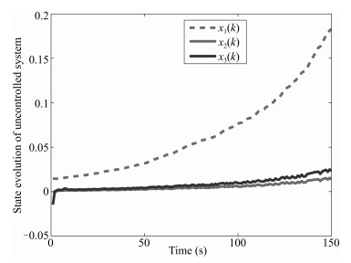 图 2 State evolution $x(k)$ of uncontrolled systems.Fig. 2 State evolution $x(k)$ of uncontrolled systems.
 图 3 State evolution $x(k)$ of controlled systems.Fig. 3 State evolution $x(k)$ of controlled systems.
In order to illustrate the disturbance-attenuation performance, we take the external disturbance
$ \begin{align*} v(k)= \begin{cases} 0.3,&20\leq k\leq 30 \\ -0.2,&50\leq k\leq 60 \\ 0,&\hbox{else}. \end{cases} \end{align*} $
Fig. 4 presents the controller-state evolution $x_c(k)$, Fig. 5 plots the state evolution of the controlled output $z(k)$, and Fig. 6 shows the output feedback controller. From Figs. 3$-$6, one can see that the convergence rate is rapid and effective. By the above simulation results, we can draw the conclusion that our theoretical analysis to the robust $H_\infty$ fuzzy-control problem is right completely.
Remark 2: The above simulation is performed on the basis of the software MATLAB 7.0 and the cone-complementarity linearization algorithm may takes several minutes because of choosing initial feasible set.
6. Conclusion
In this paper, we establish general networked systems model with multiple time-varying random communication delays and multiple missing measurements as weil as the random missing control and discuss its robust $H_\infty$ fuzzy-output feedback-control problem. The proposed system model includes parameter uncertainties, multiple stochastic time-varying delays, multiple missing measurements, and stochastic control input missing. The control strategy adopts the parallel distributed compensation. We obtain the sufficient conditions on the robustly exponential stability of the closed-loop T-S fuzzy-control system by using the CCL algorithm and the explicit expression of the desired controller parameters. An illustrative simulation example further shows that the fuzzy-control method to the proposed new control model is feasible and the new control model can be used for future applications. Whether to construct piecewise Lyapunov functions [8] to solve the proposed control model or not is an interesting topic and in active thought.
-

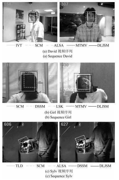
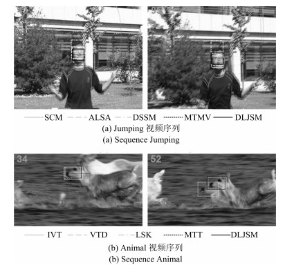
图 5 目标的光流与尺度发生剧烈变化时的跟踪结果
Fig. 5 Tracking results when targets undergo drastic changes of illumination and scale
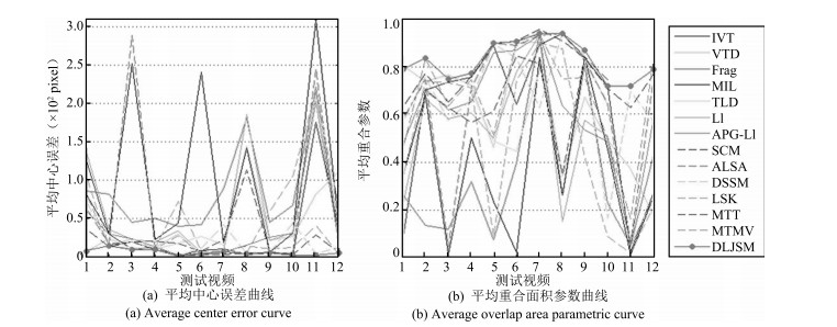
图 10 所有跟踪方法在全部测试视频上的跟踪性能
Fig. 10 Performance of all the tracking methods in test sequences
表 1 DLJSM算法与非稀疏跟踪方法的结果对比
Table 1 Comparison of the results between DLJSM algorithm and the methods not based on sparse representation
中心误差(pixel) F -参数 IVT VTD Frag MIL TLD DLJSM IVT VTD Frag MIL TLD DLJSM Girl 29.6 23.8 81.6 31.3 - 14.4 0.703 0.740 0.134 0.681 - 0.836 Singerl 9.1 3.7 42.1 241.0 27.5 3.2 0.642 0.898 0.394 0.021 0.444 0.904 Faceocc ll.2 9.5 89.5 18.6 16.0 6.3 0.891 0.903 0.940 0.838 0.786 0.938 Car4 4.0 144.8 180.5 142.1 - 4.5 0.937 0.341 0.263 0.262 - 0.939 Sylv 5.9 21.5 45.1 6.9 5.6 5.1 0.837 0.672 0.809 0.837 0.835 0.867 Race 176.4 82.2 221.4 310.6 - 2.7 0.025 0.372 0.053 0.013 - 0.721 Jumping 34.8 111.9 21.2 41.8 - 5.2 0.273 0.175 0.429 0.255 - 0.787 Animal 10.5 11.8 45.7 252.6 - 9.7 0.736 0.765 0.120 0.014 - 0.748  下载: 导出CSV
表 2 DLJSM算法与基于单个稀疏跟踪方法的结果对比
Table 2 Comparison of the results between DLJSM algorithm and the methods based on single sparse representation
中心误差(pixel) F -参数 l1 APG-l1 SCM ALSA LSK DLJSM l1 APG-l1 SCM ALSA LSK DLJSM Animal 23.1 23.9 20.2 289.5 10.2 9.7 0.583 0.619 0.652 0.046 0.732 0.748 David 20.1 13.7 9.8 11.4 11.8 9.3 0.605 0.652 0.759 0.707 0.713 0.772 Car11 33.7 2.9 2.1 2.3 73.3 2.0 0.501 0.857 0.895 0.897 0.09 0.897 Singer1 5.6 3.8 3.7 5.1 7.7 3.2 0.780 0.870 0.910 0.887 0.742 0.904 Race 214.7 203.9 28.7 245.5 217.2 2.7 0.049 0.059 0.628 0.062 0.017 0.721 Jumping 38.0 16.4 6.1 12.3 63.5 5.2 0.256 0.582 0.767 0.748 0.214 0.787 Skatingl 137.5 60.5 37.0 64.5 106.4 8.1 0.221 0.475 0.628 0.580 0.335 0.789
下载: 导出CSV
表 3 DLJSM算法与基于联合稀疏表示跟踪方法的结果对比
Table 3 Comparison of the results between DLJSM algorithm and the methods based on joint sparse representation
中心误差(pixel) F -参数 MTT MTMV DSSM DLJSM MTT MTMV DSSM DLJSM Car11 17.4 27.7 2.0 2.0 0.612 0.514 0.896 0.897 David 21.4 10.2 10.4 9.3 0.565 0.745 0.663 0.772 Race - 41.2 4.3 2.7 - 0.163 0.695 0.721 Skatingl - 81.9 73.8 8.1 - 0.451 0.569 0.789 Animal 19.4 19.5 23.7 9.7 0.630 0.635 0.574 0.748 Stone 3.3 12.5 43.9 2.8 0.746 0.50 0.166 0.720
下载: 导出CSV
-
[1] Yilmaz A, Javed O, Shah M. Object tracking:a survey. ACM Computing Surveys (CSUR), 2006, 38(4):Article No. 13 [2] Wu Y, Lim J, Yang M H. Online object tracking:a benchmark. In:Proceedings of the 2013 IEEE Conference on Computer Vision and Pattern Recognition. Portland, USA:IEEE, 2013. 2411-2418 [3] Smeulders A W M, Chu D M, Cucchiara R, Calderara S, Dehghan A, Shah M. Visual tracking:an experimental survey. IEEE Transactions on Pattern Analysis and Machine Intelligence, 2014, 36(7):1442-1468 doi: 10.1109/TPAMI.2013.230 [4] Adam A, Rivlin E, Shimshoni I. Robust fragments-based tracking using the integral histogram. In:Proceedings of the 2006 IEEE Computer Society Conference on Computer Vision and Pattern Recognition. New York, USA:IEEE, 2006. 798-805 [5] Kwon J, Lee K M. Visual tracking decomposition. In:Proceedings of the 2010 IEEE Conference on Computer Vision and Pattern Recognition. San Francisco, USA:IEEE, 2010. 1269-1276 [6] Ross D A, Lim J, Lin R S, Yang M H. Incremental learning for robust visual tracking. International Journal of Computer Vision, 2008, 77(1-3):125-141 doi: 10.1007/s11263-007-0075-7 [7] Babenko B, Yang M H, Belongie S. Visual tracking with online multiple instance learning. In:Proceedings of the 2009 IEEE Conference on Computer Vision and Pattern Recognition. Miami FL, USA:IEEE, 2009. 983-990 [8] Kalal Z, Matas J, Mikolajczyk K. P-N learning:bootstrapping binary classifiers by structural constraints. In:Proceedings of the 2010 IEEE Conference on Computer Vision and Pattern Recognition. San Francisco, USA:IEEE, 2010. 49-56 [9] Mei X, Ling H B. Robust visual tracking using L1 minimization. In:Proceedings of the 12th IEEE International Conference on Computer Vision. Kyoto, Japan:IEEE, 2009. 1436-1443 [10] Bao C L, Wu Y, Ling H B, Ji H. Real time robust L1 tracker using accelerated proximal gradient approach. In:Proceedings of the 2012 IEEE Conference on Computer Vision and Pattern Recognition. Providence, USA:IEEE, 2012. 1830-1837 [11] Zhang S P, Yao H X, Zhou H Y, Sun X, Liu S H. Robust visual tracking based on online learning sparse representation. Neurocomputing, 2013, 100:31-40 doi: 10.1016/j.neucom.2011.11.031 [12] Wang D, Lu H C, Yang M H. Online object tracking with sparse prototypes. IEEE Transactions on Image Processing, 2013, 22(1):314-325 doi: 10.1109/TIP.2012.2202677 [13] Wang L F, Yan H P, Lv K, Pan C H. Visual tracking via kernel sparse representation with multikernel fusion. IEEE Transactions on Circuits and Systems for Video Technology, 2014, 24(7):1132-1141 doi: 10.1109/TCSVT.2014.2302496 [14] Liu B Y, Huang J Z, Yang L, Kulikowsk C. Robust tracking using local sparse appearance model and k-selection. In:Proceedings of the 2011 IEEE Conference on Computer Vision and Pattern Recognition. Providence, USA:IEEE, 2011. 1313-1320 [15] Jia X, Lu H C, Yang M H. Visual tracking via adaptive structural local sparse appearance model. In:Proceedings of the 2012 IEEE Conference on Computer Vision and Pattern Recognition. Providence, USA:IEEE, 2012. 1822-1829 [16] Xie Y, Zhang W S, Li C H, Lin S Y, Qu Y Y, Zhang Y H. Discriminative object tracking via sparse representation and online dictionary learning. IEEE Transactions on Cybernetics, 2014, 44(4):539-553 doi: 10.1109/TCYB.2013.2259230 [17] Zhong W, Lu H C, Yang M H. Robust object tracking via sparsity-based collaborative model. In:Proceedings of the 2012 IEEE Conference on Computer Vision and Pattern Recognition. Providence, USA:IEEE, 2012. 1838-1845 [18] Zhang T Z, Ghanem B, Liu S, Ahuja N. Robust visual tracking via multi-task sparse learning. In:Proceedings of the 2012 IEEE Conference on Computer Vision and Pattern Recognition. Providence, USA:IEEE, 2012. 2042-2049 [19] Hong Z B, Mei X, Prokhorov D, Tao D C. Tracking via robust multi-task multi-view joint sparse representation. In:Proceedings of the 2013 IEEE International Conference on Computer Vision. Sydney, NSW:IEEE, 2013. 649-656 [20] Dong W H, Chang F L, Zhao Z J. Visual tracking with multifeature joint sparse representation. Journal of Electronic Imaging, 2015, 24(1):013006 doi: 10.1117/1.JEI.24.1.013006 [21] Zhuang B H, Lu H C, Xiao Z Y, Wang D. Visual tracking via discriminative sparse similarity map. IEEE Transactions on Image Processing, 2014, 23(4):1872-1881 doi: 10.1109/TIP.2014.2308414 [22] Zhang T Z, Liu S, Xu C S, Yan S C, Ghanem B, Ahuja N, Yang M H. Structural sparse tracking. In:Proceedings of the 2015 IEEE Conference on Computer Vision and Pattern Recognition. Boston, MA, USA:IEEE, 2015. 150-158 [23] 王梦.基于复合稀疏模型的多任务视频跟踪算法研究[硕士学位论文], 上海交通大学, 中国, 2014.Wang Meng. Multi-Task Visual Tracking Using Composite Sparse Model[Master dissertation], Shanghai Jiao Tong University, China, 2014. [24] Yuan X T, Liu X B, Yan S C. Visual classification with multitask joint sparse representation. IEEE Transactions on Image Processing, 2012, 21(10):4349-4360 doi: 10.1109/TIP.2012.2205006 [25] Doucet A, de Freitas N, Gordon N. Sequential Monte Carlo Methods in Practice. New York:Springer-Verlag, 2001. [26] Zhang T Z, Liu S, Ahuja N, Yang M H, Ghanem B. Robust visual tracking via consistent low-rank sparse learning. International Journal of Computer Vision, 2015, 111(2):171-190 doi: 10.1007/s11263-014-0738-0 期刊类型引用(4)
1. 练红海,肖伸平,罗毅平,周笔锋. 基于T-S模糊模型的采样系统鲁棒耗散控制. 自动化学报. 2022(11): 2852-2862 .  本站查看
本站查看2. 顾晓清,倪彤光,张聪,戴臣超,王洪元. 结构辨识和参数优化协同学习的概率TSK模糊系统. 自动化学报. 2021(02): 349-362 . 本站查看3. 李军,黄卫剑,万文军,刘哲. 一种新型反馈控制器的研究与应用. 控制理论与应用. 2020(02): 411-422 . 百度学术4. 唐晓铭,邓梨,虞继敏,屈洪春. 基于区间二型T-S模糊模型的网络控制系统的输出反馈预测控制. 自动化学报. 2019(03): 604-616 . 本站查看其他类型引用(1)
-

 下载:
下载:


计量
- 文章访问数: 3187
- HTML全文浏览量: 203
- PDF下载量: 843
- 被引次数: 5
