

Minimal Solution to Extrinsic Calibration of Camera and 2D Laser Rangefinder Based on Virtual Trihedron
-
摘要: 摄像机与激光测距仪(Camera and laser rangefinder, LRF)被广泛应用于机器人、移动道路测量车、无人驾驶等领域. 其中, 外参数标定是实现图像与LIDAR数据融合的第一步, 也是至关重要的一步. 本文提出一种新的基于最小解(Minimal solution) 外参数标定算法, 即摄像机与激光仅需对标定棋盘格采集三次数据. 本文首次提出虚拟三面体概念, 并以之构造透视三点问题(Perspective-three-point, P3P)用以计算激光与摄像机之间的坐标转换关系.相对于文献在对偶三维空间(Dual 3D space) 中构造的P3P问题, 本文直接在原始三维空间中构造P3P问题, 具有更直观的几何意义, 更利于对P3P问题进行求解与分析. 针对P3P问题多达八组解的问题, 本文还首次提出一种平面物成像区域约束方法从多解中获取真解, 使得最小解标定法具有更大的实用性与灵活性. 实验中分别利用模拟数据与真实数据对算法进行测试.算法结果表明, 在同等输入的条件下, 本文算法性能超过文献中的算法. 本文所提的平面物成像区域约束方法能从多解中计算出真解, 大大提高了最小解算法的实用性与灵活性.Abstract: Camera and laser rangefinder (LRF) are widely utilized in various applications, such as robotics, road survey and mapping vehicle, autonomous driving, etc. This paper presents a novel minimal solution based method for extrinsic calibration of a camera and a 2D LRF by introducing a virtual trihedron from 3 input chessboard planes. We formulate the perspective-three-plane (P3P) problem with the virtual trihedron to compute the extrinsic parameters between the camera and the LRF coordinate systems. Compared to the P3P problem in dual 3D space in existing methods, the proposed P3P problem is directly formulated in the primal 3D space, which is more intuitive and straightforward to derive and analyze the solutions. This paper also presents a novel geometric constraint, called restricted area on plane image (RAPI), to derive the unique real solution from up to 8 solutions. Results of both simulation and real data experiment demonstrate that the proposed method outperforms existing methods in terms of the same input image and LIDAR data. Moreover, the proposed method can derive the real solution from multiple solutions, thus making the minimal solution based method more practical and flexible.
-
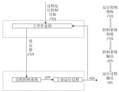
工业过程运行反馈控制包括底层回路关键被控变量的反馈控制和上层运行指标的反馈控制, 也就是说, 工业过程运行反馈控制不仅包括保证过程控制系统关键被控变量的跟踪控制, 而且还要选择合适的关键被控变量设定值, 实现运行指标目标值的跟踪[1].如图 1所示, 传统的工业过程运行反馈控制过程中, 关键被控变量的设定值$ {Y^*} = y_j^*$, $j=1, 2$, $\cdots$, $n$由工序作业班的运行工程师根据运行指标目标值${R^*} = R_i^*$, $j=1, 2, \cdots, m$和多年积累的人工操作经验, 并结合各种运行工况信息人为给出.为实现工业运行过程的自动控制, 自上世纪80年代末以来, 很多学者开展了工业运行过程控制方法的研究.文献[2]基于分层递阶控制的架构和多层优化理论, 提出了反馈优化控制的思想.文献[3]通过离线选择与工业过程经济效益相关的被控变量的设定值, 提出了自优化控制的概念.文献[4]将底层回路控制与过程运行优化相结合, 提出了具有两层结构的实时优化(Real time optimization, RTO)控制方法, 上层采用静态模型优化经济性能指标, 产生底层控制回路的设定值, 通过底层控制器使被控变量跟踪设定值, 从而尽可能使过程运行在经济指标目标值附近.文献[5]将RTO与模型预测控制相结合, 提出了具有三层结构的运行反馈控制方法.此外, 还有一些基于神经网络、模糊推理、案例推理等智能技术的运行反馈控制方法, 例如文献[6]将案例推理、规则推理以及神经网络相结合, 提出了工业运行过程的混合智能控制方法; 文献[7]将神经网络与模糊推理相结合, 提出了一种设定值的混合监控方法.
上述运行反馈控制方法均假设底层过程控制可以跟踪运行控制给出的设定值, 没有考虑底层跟踪设定值的动态误差对整个运行过程优化和控制的影响.为解决这一问题, 文献[8-9]提出了使运行指标实际值与目标值偏差和控制回路输出与设定值跟踪误差的二次性能指标极小化的运行反馈控制方法.文献[10]提出了运行反馈解耦控制方法.上述方法均假设运行层的模型由底层关键被控变量与运行指标之间的静态模型精确描述.实际上, 运行指标反映产品在加工过程中的质量、效率、消耗等, 与底层控制回路的被控变量之间往往具有动态特性, 并且很难用精确的数学模型描述.
本文针对一类运行层为未知动态模型的工业运行过程, 提出一种新的多模型自适应控制方法.最早的多模型自适应控制方法通过线性模型和基于神经网络的非线性模型之间的切换不仅可以保证自适应系统有界输入和有界输出(Bound-input and bound-output, BIBO)稳定, 而且可以改善系统的跟踪性能[11], 但该方法只适用于单输入、单输出系统, 并且是在系统的未建模动态全局有界这一假设下实现的.文献[12]将上述方法推广到多变量系统, 提出了基于多模型与神经网络的多变量自适应控制方法, 放松了文献[11]对系统未建模动态全局有界的假设.文献[13-14]提出了多变量强耦合系统的多模型自适应解耦控制方法.文献[15]提出了参数跳变系统的多模型自适应控制方法.文献[16]提出了具有未知执行器非线性的多变量自适应控制方法.
上述多模型自适应控制方法都是针对底层被控对象设计的.这些方法采用带死区的投影算法对未知参数进行在线辨识.投影算法收敛速度慢, 对参数初值十分灵敏, 实际使用中只有当参数初值接近真值时, 才具有良好的收敛效果, 因此投影算法对过程的先验知识要求较高, 不适合应用于动态未知的工业运行过程.相比较, 递推最小二乘算法具有较快的收敛速度, 对参数初值不灵敏.本文提出的运行过程多模型自适应控制方法采用带死区的递推最小二乘方法对未知参数进行在线辨识.理论分析和仿真实验验证了所提方法的有效性.
1. 问题描述
工业运行过程动态模型由上层运行层的动态模型和底层被控对象的动态模型两部分组成.在本文中, 为了将问题简化, 底层被控对象由如下离散时间线性状态空间模型描述.
$ x(k+1)=\bar{A}x(k)+\bar{B}u(k) $
(1a) $ y(k)=\bar{C}x(k) $
(1b) 其中, $x\in{\bf R}^n$为被控对象状态, $u\in{\bf R}^m$为被控对象的控制输入, $y\in{\bf R}^m$是被控对象的测量输出, $\overline{A}$ $\in$ ${\bf R}^{n\times n}$, $\overline{B}\in{\bf R}^{n\times m}$, $\overline{C}\in{\bf R}^{m\times n}$为时不变矩阵.针对底层被控对象(1)设计极点配置控制器.
$ u(k)=-Kx(k)+L{{y}^{*}}(k) $
(2) 其中, $y^{*}(k)$为底层回路设定值, $K\in{\bf R}^{m\times n}$, $L$ $\in$ ${\bf R}^{m\times m}$为时不变矩阵.
为获得控制器参数矩阵$K$和$L$, 将式(2)代入式(1)得到闭环系统方程为
$ x(k+1)=(\bar{A}-\bar{B}K)x(k)+\bar{B}L{{y}^{*}}(k) $
(3a) $ y(k)=\bar{C}x(k) $
(3b) 为使闭环系统稳定, 并实现稳态跟踪, 应选择控制器参数矩阵和满足:
1) 矩阵$\overline{A}-\overline{B}K$稳定;
2) $\lim\nolimits_{z\rightarrow1}\overline{C}(zI_{n}-(\overline{A}-\overline{B}K))^{-1}\overline{B}L=I_{m}$, $L=$ $\lim\nolimits_{z\rightarrow1}(\overline{C}(zI_{n}- (\overline{A}-\overline{B}K))^{-1}\overline{B})^{-1}$.
由于上层运行层动态模型是底层关键被控变量与运行指标之间的函数, 它的输出与底层控制系统输出相关.在本文中, 考虑运行层模型为如下带有未建模动态的动态模型.
$ r(k+1)=Mr(k)+Ny(k)+\nu (k) $
(4) 其中, $r(k)$为运行过程输出, 即运行过程的工艺指标, $\nu(k)\in {\bf R}^m$为外部干扰或未建模动态, $M$, $N$ $\in$ ${\bf R}^{m\times m}$为时不变矩阵.工业过程运行控制系统涉及到底层关键被控变量的反馈控制和上层运行指标的反馈控制, 为充分考虑底层跟踪设定值的动态误差对整个运行过程控制的影响, 运行过程动态模型可看作是由底层基础反馈控制系统(3)和运行层动态模型(4)构成的广义模型.
$ x(k+1)=\widetilde{A}x(k)+\widetilde{B}{{y}^{*}}(k) $
(5a) $ r(k+1)=Mr(k)+\widetilde{C}x(k)+\nu (k) $
(5b) 其中, $\widetilde{A}=\bar{A}-\bar{B}K$, $\widetilde{B}=\bar{B}L, $ $\widetilde{C}=N\bar{C}, $满足${{\widetilde{C}}^{\text{T}}}\widetilde{C}$可逆.
假设 1. 未建模动态$\nu(k)$的差分项或变化率全局有界, 即对任意的$k > 0$, $\|\nu(k)-\nu(k-2)\|\leq\Gamma$, 其中, $\Gamma$为正常数.
本文的目标是将设定值$y^{*}(k)$看作控制输入, 确定一个多模型自适应控制器, 当其应用于不确定的运行过程(5)时, 闭环运行过程的输入、输出信号有界, 即闭环系统BIBO稳定, 并且运行过程输出$r(k)$尽可能跟踪事先指定的运行指标目标值$r^{*}(k)$的变化.由于未建模动态的存在, 单独使用线性控制器即使能保证闭环运行过程BIBO稳定, 也很难满足一定的跟踪性能.本文将基于带死区的递推最小二乘算法的线性鲁棒自适应控制器和具有未建模动态补偿的非线性自适应控制器与切换机制相结合, 提出的多模型自适应控制器不仅能够保证闭环运行过程BIBO稳定, 而且可使其具有良好的跟踪性能.
2. 基于带死区的递推最小二乘算法的线性鲁棒自适应控制
2.1 一步超前控制器设计
为进行控制器设计, 首先需要将广义模型(5)转化成差分方程形式, 为此引入后移算子$z^{-1}$, 于是式(5)可以重新整理为
$ A({{z}^{-1}})r(k+2)=B{{y}^{*}}(k)+C({{z}^{-1}})\nu (k+1) $
(6) 其中,
$ A({{z}^{-1}})=\widetilde{C}[{{I}_{n}}-\widetilde{A}{{z}^{-1}}]{{({{\widetilde{C}}^{\text{T}}}\widetilde{C})}^{-1}}{{\widetilde{C}}^{\text{T}}}({{I}_{m}}-M{{z}^{-1}}) $
$ B=\widetilde{C}\widetilde{B} $
$ C({z^{ - 1}}) = \widetilde C[{I_n} - \widetilde A{z^{ - 1}}]{({\widetilde C^{\rm{T}}}\widetilde C)^{ - 1}}{\widetilde C^{\rm{T}}} $
下面针对模型(6)设计一步超前控制器.引入如下一步超前最优性能指标:
$ J(k) = {\left\| {T({z^{ - 1}})r(k + 2) - R({z^{ - 1}}){r^*}(k + 2)} \right\|^2} $
(7) 其中, $r^{*}(k)=[r^{*}_{1}(k), r^{*}_{2}(k), \cdots, r^{*}_{m}(k)]^{\rm T}\in{\bf R}^m$为已知有界的运行指标目标值, $T(z^{-1})\in{\bf R}^{m\times m}$为稳定的对角加权多项式矩阵, 满足$T(0)$非奇异; $R(z^{-1})$ $\in$ ${\bf R}^{m\times m}$为对角加权多项式矩阵.引入方程
$ T({z^{ - 1}}) = H({z^{ - 1}})A({z^{ - 1}}) + {z^{ - 2}}G({z^{ - 1}}) $
(8) 为使$H(z^{-1})$和$G(z^{-1})$为唯一解或最小阶解, 由文献[17]可知, $H(z^{-1})$和$G(z^{-1})$都为1阶多项式矩阵, $T(z^{-1})$的阶次小于或等于3.易知, $H(0)=T(0)$.将式(6)两边乘$H(z^{-1})$并利用式(8), 得
$ \begin{array}{l} T({z^{ - 1}})r(k + 2) = G({z^{ - 1}})r(k) + \\ \;\;\;\;\;\;H({z^{ - 1}})B{y^*}(k) + H({z^{ - 1}})C({z^{ - 1}})\nu (k + 1) \end{array} $
(9) 定义时滞-差分算子$\Delta=1-z^{-2}$, 则式(9)转化为
$ \begin{array}{l} T({z^{ - 1}})r(k + 2) = G({z^{ - 1}})\Delta r(k) + \\ \;\;\;\;\;H({z^{ - 1}})B\Delta {y^*}(k) + T({z^{ - 1}})r(k) + \rho (k) \end{array} $
(10) 其中, $\rho(k)=H(z^{-1})C(z^{-1})[\nu(k+1)-\nu(k-1)]$.于是, 使性能指标(7)最小的一步超前最优控制$y^{*}(k)$通过下式计算.
$ \begin{array}{l} G({z^{ - 1}})\Delta r(k) + H({z^{ - 1}})B\Delta {y^*}(k) + \rho (k) = \\ \;\;\;\;\;\;R({z^{ - 1}}){r^*}(k + 2) - T({z^{ - 1}})r(k) \end{array} $
(11) 将式(11)代入模型(6), 得到运行过程闭环方程
$ T({z^{ - 1}})r(k + 2) = R({z^{ - 1}}){r^*}(k + 2) $
(12) 由式(12)可知, 若选择$R(z^{-1})=T(z^{-1})$, 则可消除运行过程的跟踪误差.
由于外部干扰或未建模动态往往是未知的, 当不考虑它对运行过程闭环系统的影响时, 可采用下面的线性控制器方程求取控制输入$y^{*}(k)$.
$ \begin{array}{l} G({z^{ - 1}})\Delta r(k) + H({z^{ - 1}})B\Delta {y^*}(k) = \\ \;\;\;\;\;\;R({z^{ - 1}}){r^*}(k + 2) - T({z^{ - 1}})r(k) \end{array} $
(13) 2.2 线性鲁棒自适应控制
运行过程的动态模型往往是未知的, 因此需要采用自适应方法在线获得控制器参数, 当组成$A(z^{-1})$, $B$, $C(z^{-1})$的参数阵未知时, 式(10)可看作控制器参数辨识方程, 为此记$\phi(k)=T(z^{-1})r(k)$, $G(z^{-1})$ $=G_0+G_1(z^{-1})$, $Q(z^{-1})=H(z^{-1})B=$ $Q_0 +Q_1(z^{-1})$, 并定义数据向量和参数矩阵分别为$\varphi(k)$ $=[\Delta r^{\rm T}(k), \Delta r^{\rm T}(k-1), \Delta {y^{*}}^{\rm T}(k)$, $\Delta {y^{*}}^{\rm T}(k-1)]^{\rm T}$和$\theta=[G_0, G_1, Q_0, Q_1]^{\rm T}$, 则控制器参数辨识方程(10)可以写为
$ \phi (k + 2) = {\theta ^{\rm{T}}}\varphi (k) + \phi (k) + \rho (k) $
(14) 线性控制器方程(13)可重新写为
$ \theta^{\rm T}\varphi(k)=R(z^{-1})r^{*}(k+2)-T(z^{-1})r(k) $
(15) 对于未知的参数矩阵$\theta$, 采用带死区的递推最小二乘方法进行在线辨识.
$ \hat \theta (k) = {\rm{proj}}\{ {\hat \theta ^ + }(k)\} $
(16a) $ \begin{array}{l} {{\hat \theta }^ + }(k) = \hat \theta (k - 2){\mkern 1mu} + \\ \;\;\;\;\;\;\;\;\;\;\;\frac{{\lambda (k)P(k - 2)\varphi (k - 2){e^{\rm{T}}}(k)}}{{1 + {\varphi ^{\rm{T}}}(k - 2)P(k - 2)\varphi (k - 2)}} \end{array} $
(16b) $ \begin{array}{l} P(k) = P(k - 2) - \\ \;\;\;\;\;\;\;\;\;\;\frac{{\lambda (k)P(k - 2)\varphi (k - 2){\varphi ^{\rm{T}}}(k - 2)P(k - 2)}}{{1 + {\varphi ^{\rm{T}}}(k - 2)P(k - 2)\varphi (k - 2)}} \end{array} $
(16c) $ e(k) = \phi (k) - \hat \phi (k) $
(16d) $ \hat \phi (k) = {\hat \theta ^{\rm{T}}}(k - 2)\varphi (k - 2) + \phi (k - 2) $
(16e) $ \lambda \left( k \right) = \left\{ \begin{array}{l} \frac{1}{2}, \;\;如果\left\| {e\left( k \right)} \right\|>2E\\ 0, \;\;否则 \end{array} \right. $
(16f) $ {\rm{proj}}\left\{ {{{\hat \theta }^ + }\left( k \right)} \right\} = \left\{ \begin{array}{l} {{\hat \theta }^ + }\left( k \right), \;\;\;\;\;\;\;\;\;\;\;\;\;\hat Q_0^ + \left( k \right)非奇异\\ {\left[ { \ldots , {Q_{\min }}, \ldots } \right]^{\rm{T}}}, \;\;\;否则 \end{array} \right. $
(16g) 其中, $[\varphi(0), \widehat{\theta}(0), P(0)]$为初始条件, $P(0)>0$为正定矩阵, $E$为$\rho(k)$的已知上界, $\widehat{\theta}(k)= [\widehat{G}_0(k)$, $\widehat{G}_1(k)$, $\widehat{Q}_0(k), \widehat{Q}_1(k)]^{\rm T}$为$k$时刻未知参数矩阵$\theta$的估计, $\widehat{\theta}^{+}(k)=[\widehat{G}_0(k), \widehat{G}_1(k), \widehat{Q}_0^{+}(k), \widehat{Q}_1(k)]^{\rm T}$, ${\rm proj}\{\cdot\}$为一投影算子, 满足式(16g).
由式(15)及确定性等价原则可知, 线性鲁棒自适应控制器为
$ {\hat \theta ^{\rm{T}}}(k)\varphi (k) = R({z^{ - 1}}){r^*}(k + 2) - T({z^{ - 1}})r(k) $
(17) 2.3 线性鲁棒自适应控制系统稳定性和性能
引理 1. 定义函数
$ V(k) = {\rm{tr}}\left[ {{{\widetilde \theta }^{\rm{T}}}(k){P^{ - 1}}(K)\widetilde \theta (k)} \right] $
则带死区的递推最小二乘辨识算法(16)具有如下性质:
1)
$ \begin{array}{l} V(k) - V(k - 2) \le \\ \;\;\;\; - \frac{{3\lambda (k){{\left\| {e(k)} \right\|}^2}}}{{8[1 + {\varphi ^{\rm{T}}}(k - 2)P(k - 2)\varphi (k - 2)]}} - \\ \;\;\;\;\frac{{\lambda (k)[{{\left\| {e(k)} \right\|}^2} - 4{E^2}]}}{{4\{ 1 + [1 - \lambda (k)]{\varphi ^{\rm{T}}}(k - 2)P(k - 2)\varphi (k - 2)\} }} \end{array} $
2)
$ \mathop {\lim }\limits_{k \to \infty } \left\| {\hat \theta (k) - \hat \theta (k - 2)} \right\| = 0 $
证明. 见附录A.
定理 1. 运行过程动态模型(5)或(6)满足假设1, 则当线性鲁棒自适应控制算法(16)应用于式(6)时, 闭环运行过程全局李雅普诺夫稳定, 并且广义跟踪误差满足${\lim _{k \to \infty }}\lambda (k)[{\left\| {\bar e(k)} \right\|^2} - 4{E^2}] = 0$, 其中, $\bar e(k): = T({z^{ - 1}})r(k) - R({z^{ - 1}}){r^*}(k)$.
证明. 由引理1的1)可知,
$ \mathop {\lim }\limits_{k \to \infty } \frac{{\lambda (k)[{{\left\| {e(k)} \right\|}^2} - 4{E^2}]}}{{4\{ 1 + [1 - \lambda (k)]{\varphi ^{\rm{T}}}(k - 2)P(k - 2)\varphi (k - 2)\} }} = 0 $
(18) 由于$\overline{e}(k):=T(z^{-1})r(k)-R(z^{-1})r^*{(k)}$及$T(z^{-1})$的稳定性, 存在正常数$c_1$, $c_2$, $c_3$, $c_4$满足
$ \begin{array}{l} |{r_i}(k)| \le {c_1} + {c_2}\mathop {\max }\limits_{_{\scriptstyle0 \le \tau \le t\atop \scriptstyle1 \le i \le m}} |{{\bar e}_i}(\tau )|, \\ \;\;\;\;\;\;\;\;\;\;\;\;\;\;\;\;\;\;\;\;\;\;\;i = 1, 2, \cdots , m \end{array} $
(19) $ \begin{array}{l} |y_i^*(k - 2)| \le {c_3} + {c_4}\mathop {\max }\limits_{_{\scriptstyle0 \le \tau \le t\atop \scriptstyle1 \le i \le m}} |{r_i}(\tau )|, \\ \;\;\;\;\;\;\;\;\;\;\;\;\;\;\;\;\;\;\;\;\;\;\;\;\;i = 1, 2, \cdots , m \end{array} $
(20) 令
$ \begin{array}{l} X(k - 2) = \\ \;\;\;{[{r^{\rm{T}}}(k - 2), {r^{\rm{T}}}(k - 3), {y^*}^{\rm{T}}(k - 2), {y^*}^{\rm{T}}(k - 3)]^{\rm{T}}} \end{array} $
则存在正常数$c_5$, $c_6$满足
$ \left\| {X(k - 2)} \right\| \le {c_5} + {c_6}\mathop {\max }\limits_{0 \le \tau \le t} \left\| {\bar e(\tau )} \right\| $
(21) 由式(16d)可知,
$ e(k)=T(z^{-1})r(k)-R(z^{-1})r^{*}(k)=\overline{e}(k) $
(22) 因此, 由式(21)和式(22)可知
$ \left\| {X(k - 2)} \right\| \le {c_5} + {c_6}\mathop {\max }\limits_{0 \le \tau \le t} \left\| {e(\tau )} \right\| $
(23) 由式(23)可知, 单独采用线性鲁棒自适应控制算法时, 系统输入和输出信号的有界性由$e(k)$的有界性决定.下面假设$e(k)$无界.由式(16f)可知, 存在时刻$K_0>0$, 当$k>K_0$时, $\left\| {\mathit{e}(\mathit{k})} \right\| > {\rm{2}}E$并且$\lambda(k)$ $=$ $1/2$, 即式(18)的分子是一个正实序列.于是存在一单调递增序列$\left\| {\mathit{e}({\mathit{k}_n})} \right\|$, 使得
$ {\lim _{k \to \infty }}\left\| {e({k_n})} \right\| = \infty $
由式(23)可知
$ \begin{array}{l} \frac{{\lambda ({k_n})[{{\left\| {e({k_n})} \right\|}^2} - 4{E^2}]}}{{41 + [1 - \lambda ({k_n})]{\varphi ^{\rm{T}}}({k_n} - 2)P({k_n} - 2)\varphi ({k_n} - 2)}} \ge \\ \frac{{\lambda ({k_n})[{{\left\| {e({k_n})} \right\|}^2} - 4{E^2}]}}{{81 + [1 - \lambda ({k_n})][{{({c_5} + {c_6}\left\| {e({k_n})} \right\|)}^2}]\left\| {P({k_n} - 2)} \right\|}} \end{array} $
由于$\left\| {\mathit{P}({\mathit{k}_n} - {\rm{2}})} \right\|$为递减序列, 因此,
$ \left\| {P({k_n} - 2)} \right\| \le \left\| {P(0)} \right\| $
因此
$ \begin{array}{l} \mathop {\lim }\limits_{k \to \infty } \frac{{\lambda ({k_n})[{{\left\| {e({k_n})} \right\|}^2} - 4{E^2}]}}{{41 + [1 - \lambda ({k_n})]{\varphi ^{\rm{T}}}({k_n} - 2)P({k_n} - 2)\varphi ({k_n} - 2)}} \ge \\ \;\;\;\;\;\frac{1}{{8{c_6}\left\| {P(0)} \right\|}} > 0 \end{array} $
这与式(18)矛盾.故假设不成立, $e(k)$有界, 从而采用线性鲁棒自适应控制算法时, 闭环系统BIBO稳定.
注释 1. 单独使用线性鲁棒自适应控制器能够保证闭环运行过程全局李亚普洛夫稳定, 但是无法使运行过程具有良好的跟踪性能.为了改善运行过程的跟踪性能, 同时不影响其稳定性, 我们将线性鲁棒自适应控制器、基于神经网络的非线性控制器以及切换机制相结合, 提出一种新的多模型自适应控制方法.
3. 多模型自适应控制
3.1 多模型自适应控制算法
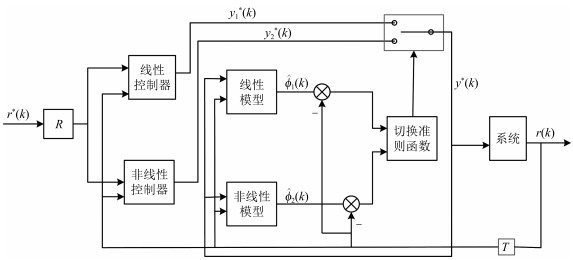
下面考虑多模型自适应控制问题, 为将问题简化, 采用两个模型, 多模型切换系统如图 2所示.
图 2中, 线性估计模型定义为
$ \widehat{\phi}_1(k)=\widehat{\theta}_1^{\rm T}(k-2)\varphi(k-2)+\phi(k-2) $
(24) 其中, $\widehat{\theta}_1(k)=[\widehat{G}_{1, 0}(k), \widehat{G}_{1, 1}(k), \widehat{Q}_{1, 0}(k), \widehat{Q}_{1, 1}(k)]^{\rm T}$为$k$时刻的基于线性模型(24)的估计, 采用式(16)在线辨识, 线性辨识误差为
$ {e_1}(k) = \phi (k) - {\hat \phi _1}(k) $
(25) 通过下式计算控制输入$y^*(k)$, 作为基于线性模型的控制器$y^*_1(k)$.
$ \hat \theta _1^{\rm{T}}(k)\varphi (k) = R({z^{ - 1}}){r^*}(k + 2) - T({z^{ - 1}})r(k) $
(26) 非线性估计模型定义为
$ {\hat \phi _2}(k) = \hat \theta _2^{\rm{T}}(k - 2)\varphi (k - 2) + \phi (k - 2) + \hat \rho (k - 2) $
(27) 其中,$\widehat{\theta}_2(k)=[\widehat{G}_{2, 0}(k), \widehat{G}_{2, 1}(k), \widehat{Q}_{2, 0}(k), \widehat{Q}_{2, 1}(k)]^{\rm T}$为$k$时刻$\theta$的基于非线性模型(27)的估计; $\widehat{\rho}(k)$为$\rho^*(k)$的神经网络估计, 其中, $\rho^*(k):=\Delta\phi(k+2)-\widehat{\theta}_2(k)^{\rm T}\varphi(k)$, 即
$ \widehat{\rho}(k)=NN[\widehat{W}(k), \varphi(k)] $
(28) 其中, $NN[\cdot]$表示神经网络结构; $\varphi(k)$为神经网络的输入向量; $\widehat{W}(k)$为$k$时刻理想权阵$W^*$的估计.与文献[12]类似, 除了要求参数阵的估计$\widehat{\theta}_2(k)$和权阵的估计$\widehat{W}(k)$有界, $\widehat{Q}_{2, 0}(k)$非奇异, 并未对$\widehat{\theta}_2(k)$的辨识算法和神经网络的结构以及权阵校正算法进行任何限制, 即
$ \widehat{\theta}_2(k), \widehat{W}(k);~~\widehat{Q}_{2, 0}(k)~\text{非奇异}, ~ \forall k $
(29) 非线性辨识误差为
$ e_2(k)=\phi(k)-\widehat{\phi}_2(k) $
(30) 因此, 根据式(10)和确定性等价原则, 通过下式计算控制输入$y^*(k)$, 作为基于非线性模型的控制器$y^*_2(k)$.
$ \begin{array}{l} {{\hat \theta }_2}(k)\varphi (k) + \hat \rho (k) = R({z^{ - 1}}){r^*}(k + 2){\mkern 1mu} - \\ \;\;\;\;\;\;\;\;T({z^{ - 1}})r(k) \end{array} $
(31) 切换准则为
$ \begin{array}{l} {J_j}\left( k \right) = \sum\limits_{i = 2}^k {\frac{{{\lambda _j}(k)[{{\left\| {{e_j}(k)} \right\|}^2} - 4{E^2}]}}{{4\{ 1 + [1 - {\lambda _j}(k)]{\varphi ^{\rm{T}}}(k - 2)P(k - 2)\varphi (k - 2)\} }} + } \\ {c_0}\sum\limits_{l = k - N - 1}^k {\left( {\frac{1}{2} - {\lambda _j}(l){{\left\| {{e_j}(l)} \right\|}^2}} \right)} \end{array} $
(32) $ {\lambda _j}\left( k \right) = \left\{ \begin{array}{l} \frac{1}{2}, \;\;若\left\| {{e_j}(k)} \right\|>2E\\ 0, \;\;否则 \end{array} \right. $
(33) 其中, $N$是一个正整数, $c_0$是一个大于等于0的预先确定的常数.
每一时刻$k$, 比较$J_1(k)$和$J_2(k)$, 求出最小的$J^*(k)$, 选择与$J^*(k)$对应的自适应控制器$y_i^*(k)$, 并将其应用于运行过程.
3.2 多模型自适应控制系统稳定性和性能
定理 2. 运行过程动态模型(6)满足假设1, 则当基于多模型自适应控制算法(24)~ (33)用于运行过程(6)时, 闭环切换系统BIBO稳定.此外, 对于任意给定的正数$\varepsilon$, 存在时刻$K$, 当$k>K$时, 系统的广义跟踪误差满足$\left\| {\bar e(k)} \right\| \le 2E + \varepsilon $.
证明. 由引理1可知,
$ \mathop {\lim }\limits_{k \to \infty } \frac{{{\lambda _1}(k)[{{\left\| {{e_1}(k)} \right\|}^2} - 4{E^2}]}}{{4\{ 1 + [1 - {\lambda _1}(k)]{\varphi ^{\rm{T}}}(k - 2)P(k - 2)\varphi (k - 2)\} }} = 0 $
(34) 由式(24)和式(25)可知,
$ \begin{array}{l} {e_1}(k) = \phi (k) - {{\hat \phi }_1}(k) = \\ \;\;\;\;\;\;\;\;\;\;\Delta \phi (k) - \hat \theta _1^{\rm{T}}(k - 2)\varphi (k - 2) = \\ \;\;\;\;\;\;\;\;\;T({z^{ - 1}})r(k) - T({z^{ - 1}})r(k - 2) - \\ \;\;\;\;\;\;\;\;\hat \theta _1^{\rm{T}}(k - 2)\varphi (k - 2) \end{array} $
(35) 由式(27)和式(30)可知
$ \begin{array}{l} {e_2}(k) = \phi (k) - {{\hat \phi }_2}(k) = \\ \;\;\;\;\;\;\Delta \phi (k) - \hat \theta _2^{\rm{T}}(k - 2)\varphi (k - 2) - \hat \rho (k - 2) = \\ \;\;\;\;\;\;T({z^{ - 1}})r(k) - T({z^{ - 1}})r(k - 2) - \\ \;\;\;\;\;\;\hat \theta _2^{\rm{T}}(k - 2)\varphi (k - 2) - \hat \rho (k - 2) \end{array} $
(36) 于是, 根据确定性等价原则, 每一时刻
$ \bar{e}(k)=e_1(k)~ \mbox{或}~e_2(k) $
(37) 由于每一时刻, 系统辨识误差$e(k)=e_1(k)$或$e_2(k)$, 故由式(21)可知, 存在正常数$c_7$, $c_8$满足
$ \left\| {X(k - 2)} \right\| \le {c_7} + {c_8}\mathop {\max }\limits_{0 \le \tau \le k} \left\| {e(\tau )} \right\| $
(38) 由式(33)可知, 切换函数$J_j(k)$ $(j=1, 2)$的第2项是有界的.因此由引理1可知, $J_1(k)$有界.对于$J_2(k)$有两种情况.
1) $J_2(k)$无界.由于$J_1(k)$有界, 因此存在时刻$K_1$使得当$k\geq K_1$时有$J_1(k)\leq J_2(k)$.故根据切换机制, 当$k\geq K_1+1$时, 系统辨识误差$e(k)=e_1(k)$满足
$ \mathop {\lim }\limits_{k \to \infty } \frac{{{\lambda _1}(k)[{{\left\| {e(k)} \right\|}^2} - 4{E^2}]}}{{4\{ 1 + [1 - {\lambda _1}(k)]{\varphi ^{\rm{T}}}(k - 2)P(k - 2)\varphi (k - 2)\} }} = 0 $
(39) 其中,
$ \lambda \left( k \right) = \left\{ \begin{array}{l} \frac{1}{2}, \;\;若\left\| {e(k)} \right\|>2E\\ 0, \;\;否则 \end{array} \right. $
2) $J_2(k)$有界.由切换准则式(32)可知, $e_2(k)$满足
$ \mathop {\lim }\limits_{k \to \infty } \frac{{{\lambda _2}(k)[{{\left\| {{e_2}(k)} \right\|}^2} - 4{E^2}]}}{{4\{ 1 + [1 - {\lambda _2}(k)]{\varphi ^{\rm{T}}}(k - 2)P(k - 2)\varphi (k - 2)\} }} \to 0 $
故系统辨识误差$e(k)=e_1(k)$或$e_2(k)$满足式(39).
其余部分的证明类似于定理1.
由式(39)和$X(k-2)$的有界性可知,
$ \mathop {\lim }\limits_{k \to \infty } \lambda (k)\left[ {{{\left\| {e(k)} \right\|}^2} - 4{E^2}} \right] $
即, 对任意小的正数$\varepsilon$, 存在时刻$K$, 当$k>K$时,
$ \left\| {e(k)} \right\| \le 2E + \varepsilon $
(40) 注释2. 由式(39)可知, 非线性辨识误差
$ {e_2}(k) = {\rho ^*}(k - 2) - \hat \rho (k - 2) $
(41) 适当选择神经网络结构和参数, 可以保证$\left\| {{\rho ^*}(k} \right.$ $-$ $\left. {2) - \hat \rho (k - 2)} \right\|<\varepsilon $.因此若运行过程选择非线性自适应控制器$y_2^*(k)$作为输入信号, 则由式(35)和式(36)可知, 广义跟踪误差$\left\| {\bar e(k)} \right\|<\varepsilon $满足.
4. 仿真实验
为验证本文所提方法的有效性, 首先考虑如下底层被控对象模型
$ \begin{array}{l} x(k + 1) = \left( {\begin{array}{*{20}{c}} {1.5}&6\\ 6&4 \end{array}} \right)x(k) + \\ \;\;\;\;\;\;\;\;\;\left( {\begin{array}{*{20}{c}} { - 4.2623}&{ - 3.8254}\\ {8.3534}&{6.1711} \end{array}} \right)u(k)\\ y(k) = \left( {\begin{array}{*{20}{c}} {0.1546}&{ - 0.012}\\ { - 0.0099}&{0.2281} \end{array}} \right)x(k) \end{array} $
(42) 其中, $x=[x_1, x_2]^{\rm T}$, $y=[y_1, y_2]^{\rm T}$, $u=[u_1, u_2]^{\rm T}$.为使底层闭环系统稳定, 并实现稳态跟踪, 选择如下极点配置控制器
$ u(t)=-Kx(t)+Ly^*(t) $
(43) 其中, $y^*(t)=[y_1^*, y_2^*]^{\rm T}$为底层回路设定值, 由后面的运行控制给出.
$ \begin{array}{l} K = \left( {\begin{array}{*{20}{c}} {7.1487}&{15.3085}\\ { - 8.8017}&{ - 19.0044} \end{array}} \right)\\ \;\;L = \left( {\begin{array}{*{20}{c}} { - 14.5}&{30.25}\\ { - 20.6}&{ - 35.6} \end{array}} \right) \end{array} $
(44) 假设运行层动态模型为
$ \begin{array}{l} r(k + 1) = \left( {\begin{array}{*{20}{c}} 1&0\\ 0&1 \end{array}} \right)r(k) + \\ \;\;\;\;\;\;\;\;\;\;\;\;\;\;\left( {\begin{array}{*{20}{c}} { - 1.2893}&{ - 0.0678}\\ {0.2798}&{ - 4.3693} \end{array}} \right)y(k) + \nu (k) \end{array} $
(45) 其中,
$ r(k) = {[{r_1}, {r_2}]^{\rm{T}}} $
$ \begin{array}{l} \nu (k) = \left( {\begin{array}{*{20}{c}} {{\nu _1}}\\ {{\nu _2}} \end{array}} \right) = 0.01 \times \\ \;\;\;\;\;\;\;\;\;\;\left( {\begin{array}{*{20}{c}} {{\rm{sin}}({\rm{1 + }}y_{\rm{1}}^{{\rm{*2}}}(k{\rm{ - 1}}){\rm{ + }}r_{\rm{1}}^{\rm{2}}(k{\rm{ - 1}}){\rm{ + }}}\\ {r_2^2(k) - \frac{{{r_1}(k - 1) + {r_2}(k)}}{{1 + y_1^{*2}(k - 1) + r_1^2(k - 1) + r_2^2(k)}})}\\ {{\rm{sin}}({\rm{1 + }}y_{\rm{2}}^{{\rm{*2}}}(k{\rm{ - 1}}){\rm{ + }}r_{\rm{1}}^{\rm{2}}(k{\rm{ - 1}}){\mkern 1mu} {\rm{ + }}}\\ {r_2^2(k) - \frac{{{r_1}(k) + {r_2}(k - 1)}}{{1 + y_2^{*2}(k - 1) + r_1^2(k) + r_2^2(k - 1)}})} \end{array}} \right) \end{array} $
则由式(5)可知, 运行过程广义对象模型为
$ \begin{array}{l} x(k + 1) = \left( {\begin{array}{*{20}{c}} { - 1.7}&{ - 1.45}\\ {0.6}&{ - 6.6} \end{array}} \right)x(k) + \\ \;\;\;\;\;\;\;\;\;\;\;\;\;\;\left( {\begin{array}{*{20}{c}} {17}&{7.25}\\ { - 6}&{33} \end{array}} \right){y^*}(k)\\ r(k + 1) = \left( {\begin{array}{*{20}{c}} 1&0\\ 0&1 \end{array}} \right)r(k) + \\ \;\;\;\;\;\;\;\;\;\;\;\;\;\;\left( {\begin{array}{*{20}{c}} { - 0.2}&0\\ 0&{ - 1} \end{array}} \right)x(k) + \nu (k) \end{array} $
(46) 选择加权多项式矩阵
$ \begin{array}{l} T({z^{ - 1}}) = R({z^{ - 1}}) = \\ \;\;\;\;\;\;\;\;\;\;\;\;\left( \begin{array}{l} - 5 - 0.1{z^{ - 1}}\;\;\;\;\;\;\;\;\;0\\ \;\;\;\;\;\;0\;\;\;\;\;\;\;\;\; - 1 - 0.1{z^{ - 1}} \end{array} \right) \end{array} $
运行指标目标值为
$ {r^*}(k) = \left( \begin{array}{l} \;\;\;\;\;\;\;\;\;\;\;\;\;0.5\\ 0.5{\rm{sign}}\left( {\cos \left( {k \times \frac{\pi }{{50}}} \right)} \right) \end{array} \right) $
易知, 控制器真实参数阵为
$ \theta = \left( {{\theta _0}\;\;\;\;\;{\theta _1}} \right) $
其中,
$ \begin{array}{l} {\theta _0} = ( - 6.53, - 10.556, 1.43, 10.556, 17, 7.25, \\ \;\;\;\;\;\;\;\; - 2.86, - 52.78{)^{\rm{T}}} \end{array} $
$ \begin{array}{l} {\theta _1} = (21.6, - 36.53, - 21.6, 35.43, - 6, 33, \\ \;\;\;\;\;\;\;43.2, - 177.15{)^{\rm{T}}} \end{array} $
本仿真实验中, 我们假设它是未知的, 并根据先验知识选择待辨识控制器初始参数阵为
$ \begin{array}{l} \\ \begin{array}{*{20}{l}} {\hat \theta (0) = {{\left( {\begin{array}{*{20}{c}} { - 4}&{ - 7}&0&4&{19}&3&{ - 1}&{ - 35}\\ {16}&{ - 31}&{ - 15}&{30}&{ - 2}&{29}&{35}&{ - 160} \end{array}} \right)}^{\rm{T}}}} \end{array} \end{array} $
选择单隐层线性输出的静态BP网对$\rho^*(k)$进行估计, 其隐元数为20, 学习率为0.1;选择$c=1$, $N$ $=$ $2$.
图 3为单独采用线性鲁棒自适应控制方法时运行过程的运行指标目标值$r^*(k)$和运行过程输出$r(k)$.从图 3可以看出, 虽然该控制器可以使运行过程稳定, 但跟踪效果很差. 图 4为采用本文所提的多模型自适应控制方法时运行过程的运行指标目标值$r^*(k)$、运行过程输出$r(k)$和运行过程控制输入, 即底层设定值$y^*(k)$.与图 3相比, 图 4中的跟踪效果明显改善. 图 5为$\widehat{\theta}_1(k)$中16个参数的在线变化曲线. 图 6为底层极点配置控制系统的跟踪曲线.为进行比较, 仍以上述矩阵为控制器初始参数阵, 采用文献[12]提出的基于投影算法的多模型自适应控制方法对运行过程进行仿真, 运行过程跟踪结果如图 7所示.相应的$\widehat{\theta}_1(k)$中各参数的在线变化曲线如图 8所示.由图 4和图 7可知, 采用本文提出的基于最小二乘算法的多模型自适应控制方法时, 即使控制器初始参数阵离控制器真实参数阵较远, 仍具有有良好的跟踪效果.两相比较, 基于投影算法的多模型自适应控制方法对初始参数阵非常灵敏, 当初始参数阵远离控制器真实参数阵时, 控制效果较差.比较图 5和图 8可以看出, 最小二乘算法与投影算法相比具有更快的收敛速度.
 图 3 采用基于递推最小二乘算法的线性鲁棒自适应控制方法时, 运行过程的输出及运行指标目标值Fig. 3 Outputs of the operation process and theirs operation targets when the linear robust adaptive control method based on recursive least square algorithm is used
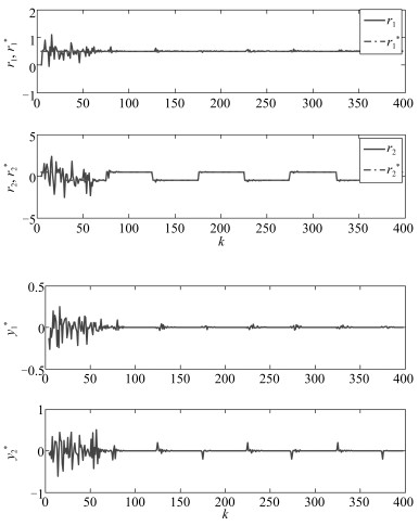 图 4 采用基于递推最小二乘算法的多模型自适应控制方法时, 运行过程的输出、运行指标目标值及控制输入Fig. 4 Outputs of the operation process, theirs operation targets and control inputs when the proposed multi-model adaptive control method based on recursive least square algorithm is used
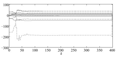 图 5 采用基于递推最小二乘算法的多模型自适应控制方法时, $\widehat{\theta}_1(k)$中16个参数的在线变化曲线Fig. 5 Online curves of 16 parameters in $\widehat{\theta}_1(k)$ when the proposed multi-model adaptive control method based on recursive least square algorithm is used
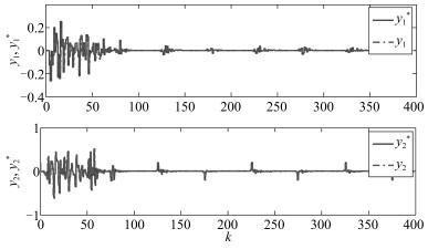 图 6 底层极点配置控制系统的跟踪曲线Fig. 6 Tracking curves of the underlying pole assignment control system
 图 7 采用基于投影算法的多模型自适应控制方法时, 运行过程的输出和运行指标目标值Fig. 7 Outputs of the operation process and theirs operation targets when the multi-model adaptive control method based on projection algorithm is used
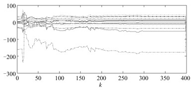 图 8 采用基于投影算法的多模型自适应控制方法时, $\widehat{\theta}_1(k)$中16个参数的在线变化曲线Fig. 8 Online curves of 16 parameters in $\widehat{\theta}_1(k)$ when the multi-model adaptive control method based on projection algorithm is used
5. 结论
工业运行过程应考虑底层跟踪设定值的动态误差对整个运行过程优化和控制的影响.现有的工业运行控制方法假设运行层为已知的线性静态模型.本文针对一类运行层为未知线性动态模型的工业运行过程, 提出了一种基于递推最小二乘算法的多模型自适应控制方法.通过理论分析和仿真比较, 验证了与现有的多模型自适应控制方法相比, 本文提出方法可以应用于工业运行过程, 并具有良好的跟踪效果.
工业过程运行控制是近年来控制领域比较热门的研究方向之一, 现有的方法针对的被控对象主要是线性的, 并且主要集中在理论研究上.在实际的工业过程控制中, 非线性动态无可避免, 当两层结构中的被控对象都是非线性时, 如何设计控制器, 如何将理论的研究成果进行实际应用具有一定的挑战.
附录A. 引理1的证明
证明. 当$\widehat{Q}_0^+(k)$非奇异时, $\widehat{\theta}(k)$与$\widehat{\theta}^+(k)$相等.由式(16d)和式(16e)可知,
$ e(k) = [{\theta ^{\rm{T}}} - {\hat \theta ^{\rm{T}}}(k - 1)]\varphi (k - 2) + \rho (k - 2) $
(A1) 令
$ L(k)=\frac{P(k-2)\varphi(k-2)}{1+\varphi^{\rm T}(k-2)P(k-2)\varphi(k-2)} $
(A2) 由式(16b)、式(16c)以及式(A1)和式(A2)可知,
$ \begin{array}{l} P(k) = P(k - 2) - \lambda (k)L(k){\varphi ^{\rm{T}}}(k - 2)P(k - 2) \Rightarrow \\ P(k) = [I - \lambda (k)L(k){\varphi ^{\rm{T}}}(k - 2)]P(k - 2) \Rightarrow \\ P(k){P^{ - 1}}(k - 2) = I - \lambda (k)L(k){\varphi ^{\rm{T}}}(k - 2) \end{array} $
(A3) 和
$ \begin{array}{l} \widetilde \theta (k) = \widetilde \theta (k - 2) + \lambda (k)L(k){e^{\rm{T}}}(k) = \\ \;\;\;\;\;\;\;\;\;\;[I - \lambda (k)L(k){\varphi ^{\rm{T}}}(k - 2)]\widetilde \theta (k - 2) + \\ \;\;\;\;\;\;\;\;\;\;\lambda (k)L(k){\rho ^{\rm{T}}}(k - 2) = \\ \;\;\;\;\;\;\;\;\;\;P(k){P^{ - 1}}(k - 2)\widetilde \theta (k - 2) + \\ \;\;\;\;\;\;\;\;\;\lambda (k)L(k){\rho ^{\rm{T}}}(k - 2) \end{array} $
(A4) 由式(A4)可知,
$ \begin{array}{l} {P^{ - 1}}(k)\widetilde \theta (k) - {P^{ - 1}}(k - 2)\widetilde \theta (k - 2) = \\ \;\;\;\;\;\;\lambda (k){P^{ - 1}}(k)L(k){\rho ^{\rm{T}}}(k - 2) \end{array} $
(A5) 由于$\varphi^{\rm T}(k-2)P(k-2)\varphi(k-2)\times I=\varphi(k-2)\varphi^{\rm T}(k-2)P(k-2)$, 因此由式(16c)可知
$ \begin{array}{l} \frac{{{P^{ - 1}}(k)P(k - 2)\varphi (k - 2)}}{{1 + {\varphi ^{\rm{T}}}(k - 2)P(k - 2)\varphi (k - 2)}} = \\ \;\;\;\;\frac{{\varphi (k - 2)}}{{1 + [1 - \lambda (k)]{\varphi ^{\rm{T}}}(k - 2)P(k - 2)\varphi (k - 2)}} \end{array} $
(A6) 令$Q(k):=\varphi^{\rm T}(k-2)P(k-2)\varphi(k-2)$, 则
$ \begin{array}{l} V(k) - V(k - 2) = \\ \;\;\;\;\;\;\;{\rm{tr}}\{ - \frac{{\lambda (k)[e(k){e^{\rm{T}}}(k) - 4\rho (k - 2){\rho ^{\rm{T}}}(k - 2)]}}{{4[1 + [1 - \lambda (k)]Q(k)]}} - \\ \;\;\;\;\;\;\;\left. {\frac{{3\lambda (k)e(k){e^{\rm{T}}}(k)[1 + Q(k)[1 - \frac{{4\lambda (k)}}{3}]]}}{{4[1 + [1 - \lambda (k)]Q(k)][1 + Q(k)]}}} \right\} \end{array} $
(A7) 由于
$ \frac{1+Q(k)\left[1-\frac{4\lambda(k)}{3}\right]}{1+[1-\lambda(k)]Q(k)}\geq \frac{1}{2} $
(A8) 因此
$ \begin{array}{l} V(k) - V(k - 2) \le \\ \;\;\;\;\;{\rm{tr}}\{ - \frac{{\lambda (k)[e(k){e^{\rm{T}}}(k){\rm{ - 4}}\rho (k{\rm{ - 2}}){\rho ^{\rm{T}}}(k{\rm{ - 2}})]}}{{{\rm{4}}[{\rm{1 + }}[{\rm{1 - }}\lambda (k)]Q(k)]}} - \\ \;\;\;\;\;\frac{{3\lambda (k)e(k){e^{\rm{T}}}(k)}}{{8[1 + Q(k)]}}\} \le \\ \;\;\;\;\; - \frac{{\lambda (k)[{{\left\| {e(k)} \right\|}^2} - 4{E^2}]}}{{4[1 + [1 - \lambda (k)]Q(k)]}} - \frac{{3\lambda (k){{\left\| {e(k)} \right\|}^2}}}{{8[1 + Q(k)]}} \end{array} $
(A9) 因此, 引理1中1)得证.由式(16b)可知,
$ \begin{array}{l} {\varphi ^{\rm{T}}}(k - 2)[\hat \theta (k) - \hat \theta (k - 2)] = \\ \;\;\;\;\;\;\frac{{\lambda (k){\varphi ^{\rm{T}}}(k - 2)P(k - 2)\varphi (k - 2){e^{\rm{T}}}(k)}}{{1 + {\varphi ^{\rm{T}}}(k - 2)P(k - 2)\varphi (k - 2)}} \end{array} $
(A10) 因此
$ \begin{array}{l} {\varphi ^{\rm{T}}}(k - 2)[\hat \theta (k) - \hat \theta (k - 2)][\hat \theta (k) - \\ \;\;\;\;\;\;\;\hat \theta (k - 2){]^{\rm{T}}}\varphi (k - 2) \le \\ \;\;\;\;\;\;\;\frac{{\lambda (k){\varphi ^{\rm{T}}}(k - 2)P(k - 2)\varphi (k - 2){e^{\rm{T}}}(k)e(k)}}{{1 + {\varphi ^{\rm{T}}}(k - 2)P(k - 2)\varphi (k - 2)}} \end{array} $
(A11) 故
$ {\left\| {\hat \theta (k) - \hat \theta (k - 2)} \right\|^2} \le \frac{{\lambda (k)\left\| {P(k - 2)} \right\|{e^{\rm{T}}}(k)e(k)}}{{1 + {\varphi ^{\rm{T}}}(k - 2)P(k - 2)\varphi (k - 2)}} $
(A12) 由引理1中的1)及$\| P(k-2)\|$的有界性, 可知2)成立.当$\widehat{Q}_0^+(k)$非奇异时, 记.由式(16g)可知${\left\| {{\theta ^ + }(k) - \theta } \right\|^2}$, 因此$V^+(k)\leq V(k)$, 故引理1\linebreak仍旧成立.
-
[1] Kassir A, Peynot T. Reliable automatic camera-laser calibration. In:Proceedings of the 2010 Australasian Conference on Robotics and Automation. Brisbane, Australia:ARAA, 2010. 1-10 [2] [2] Bosse M, Zlot R, Flick P. Zebedee:design of a spring-mounted 3-D range sensor with application to mobile mapping. IEEE Transactions on Robotics, 2012, 28(5):1104-1119 [3] [3] Osgood T J, Huang Y P. Calibration of laser scanner and camera fusion system for intelligent vehicles using Nelder-Mead optimization. Measurement Science and Technology, 2013, 24(3):1-10 [4] [4] Chen Z, Zhuo L, Sun K Q, Zhang C X. Extrinsic calibration of a camera and a laser range finder using point to line constraint. Procedia Engineering, 2012, 29:4348-4352 [5] [5] Li G H, Liu Y H, Dong L, Cai X P. An algorithm for extrinsic parameters calibration of a camera and a laser range finder using line features. In:Proceedings of the 2007 IEEE/RSJ International Conference on Intelligent Robots and Systems. San Diego, CA, United states:IEEE, 2007. 3854-3859 [6] [6] Ha J E. Extrinsic calibration of a camera and laser range finder using a new calibration structure of a plane with a triangular hole. International Journal of Control, Automation and Systems, 2012, 10(6):1240-1244 [7] [7] Kwak K, Huber D F, Badino H, Kanade T. Extrinsic calibration of a single line scanning LIDAR and a camera. In:Proceedings of the 2011 IEEE/RSJ International Conference on Intelligent Robots and Systems. San Francisco, CA, USA:IEEE, 2011. 3283-3289 [8] [8] Zhang Z Y. A flexible new technique for camera calibration. IEEE Transactions on Pattern Analysis and Machine Intelligence, 2000, 22(11):1330-1334 [9] [9] Zhang Q, Pless R. Extrinsic calibration of a camera and laser range finder (improves camera calibration). In:Proceedings of the 2004 IEEE/RSJ International Conference on Intelligent Robots and Systems. Sendai, Japan:IEEE, 2004. 2301-2306 [10] Vasconcelos F, Barreto J P, Nunes U. A minimal solution for the extrinsic calibration of a camera and a laser-rangefinder. IEEE Transactions on Pattern Analysis and Machine Intelligence, 2012, 34(11):2097-2107 [11] Fishler M A, Bolles R C. Random sample consensus:a paradigm for model fitting with applications to image analysis and automated cartography. Communications of the ACM, 1981, 24(6):381-395 [12] Zhou L P. A new minimal solution for the extrinsic calibration of a 2D LIDAR and a camera using three plane-line correspondences. IEEE Sensors Journal, 2014, 14(2):442-454 [13] Yang H, Liu X L, Patras I. A simple and effective extrinsic calibration method of a camera and a single line scanning LIDAR. In:Proceedings of the 21st International Conference on Pattern Recognition (ICPR). Tsukuba, Japan:IEEE, 2012. 1439-1442 [14] Dacorogna B, Marchal P. The role of perspective functions in convexity, poly-convexity, rank-one convexity and separate convexity. Journal of Convex Analysis, 2008, 15(2):271-284 期刊类型引用(6)
1. 陈德旺,刘俐俐,赵文迪,欧纪祥,孙艳焱,郑楠. 基于模糊系统的定性与定量知识的综合集成. 智能科学与技术学报. 2024(04): 445-455 .  百度学术
百度学术2. Hong Mo,Yinghui Meng,Fei-Yue Wang,Dongrui Wu. Interval Type-2 Fuzzy Hierarchical Adaptive Cruise Following-Control for Intelligent Vehicles. IEEE/CAA Journal of Automatica Sinica. 2022(09): 1658-1672 . 必应学术3. 曹小玲,莫红,朱凤华. 时变论域下红绿灯配时的模糊控制. 测控技术. 2019(11): 115-120 . 百度学术4. 王飞跃,魏庆来. 智能控制:从学习控制到平行控制. 控制理论与应用. 2018(07): 939-948 . 百度学术5. 莫红,刘芬. 区间二型模糊综合评判下的语言动力学分析. 模式识别与人工智能. 2018(06): 548-553 . 百度学术6. 杨乾坤,王晓红. 基于多路口预测与实时配时合作的交通控制系统设计. 计算机测量与控制. 2018(12): 93-96 . 百度学术其他类型引用(14)
-

 下载:
下载:
计量
- 文章访问数: 2002
- HTML全文浏览量: 88
- PDF下载量: 1600
- 被引次数: 20
 下载:
下载:
