

Research on Temporal Consistency and Robustness in Local Planning of Intelligent Vehicles
-
摘要: 在无人驾驶系统中,局部规划在跟踪全局路径的同时完成避障,提高了规划系统在动态未知环境中的工作能力.避障分析的有效性是局部规划最重要的功能之一.然而在仿真和实车测试中发现,广泛使用的基于优化求解的局部规划算法无法在不依赖全局精确定位时保证规划结果满足时间一致性要求.时间不一致将导致车辆的实际行驶路线偏离初始规划结果,造成避障分析失效.本文设计了基于前向预测的局部路径规划算法,在不依赖全局精确定位的前提下保证规划结果的时间一致性.除了时间一致性问题外,跟踪控制误差也是导致规划结果避障分析失效的主要原因之一.现有研究大多通过膨胀障碍物体现误差的影响,然而这种方法无法避免车辆驶入膨胀危险区域而停车.本算法在路径生成过程中增加误差影响,用通行区域代替原有不具有宽度的规划路径进行避障分析,既可以解决误差导致的避障失效,又避免出现膨胀障碍物带来的问题.通过V-Rep软件与实车规划程序进行联合仿真,在能够体现时间一致性影响的典型场景中对本算法与基于最优化曲线生成的局部路径规划算法进行比较, 验证了该算法具有更好的安全分析有效性.应用本算法的北京理工大学无人驾驶平台参加了2013年智能车未来挑战赛,在无人干预的情况下顺利完成 18公里城郊赛段和5公里城市赛段行驶,展现了良好的避障能力.Abstract: Local planner can improve the capacity of planning system for intelligent vehicles by avoiding obstacles while tracking the reference path. Safety check is the one of the fundamental functions of a local planner. However, revealed by simulation and experiments, the widely used optimization-based local planning methods are unlikely to maintain temporal consistency without any accurate global positioning information. Temporal inconsistency will result in the deviation of the vehicle's actual trajectory from the original planned results, which will finally make the safety check invalid. This paper presents a forward prediction-based local planning algorithm which holds temporal consistency in the results without requiring any accurate global positioning information. Besides the temporal consistency issue, controlling error is another reason for safety check failure. Most current researches take error into consideration by enlarging the size of obstacles. Such methods are unable to prevent the vehicle from entering the dilated obstacle areas. In this paper, controlling error is introduced in the generation of the local paths. The traditional path with no width is replaced by a strip of path here. Based on the simulation results of the V-Rep virtual reality software, the forward prediction-based method features better safety check ability as compared with the optimization-based local planning methods. The proposed algorithm was applied to the intelligent vehicle by Beijing Institute of Technology which participated in The Future Challenge 2013. The vehicle succeeded to finish the event without human operation.
-
Key words:
- Intelligent vehicle /
- local planning /
- temporary consistency /
- robustness
-
1. Introduction
Since recent few decades, some researchers focus their energy on the robust stability and controller design problems about the networked-control systems (NCSs) with some uncertain parameters because some networked-control systems have been succeeded in applications in modern complicated industry processes, e.g., aircraft and space shuttle, nuclear power stations, high-performance automobiles, etc. The fuzzy-logic control based on the Takagi-Sugeno (T-S) is widely used to dealing with complex nonlinear systems because it has simple dynamic structure and highly accurate approximation to any smooth nonlinear function in any compact set. One can consult [1]$-$[8] and the other cited literature therein [9]$-$[31]. Data-packet dropout is an important issue to be addressed in the networked-control systems [6], [32]. Zhang [33] solves the problem of $H_\infty$ estimation for a class of Markov jump linear systems but he neglect possible dropout in practice. Reference [34] reports the problem of $H_\infty$ stability of discrete-time switched linear system with average dwell time and with no dropout. In [6], piecewise Lyapunov function is proposed to analyze robust of the nonlinear NCSs without time-delay issue. Random data-packet dropout and time delay are well considered but the controlled NCSs are linear systems in [32]. Reference [8] discusses the problem of robust $H_\infty$ output feedback control for a class of continuous-time Takagi-Sugeno (T-S) fuzzy affine dynamic systems with parametric uncertainties and input constraints on ignoring some nonlinearities induced by system with data-packet dropout and random time delay. Reference [5] investigates the robust $H_\infty$ stability of a class of half nonlinear NCSs with multiple probabilistic delays and multiple missing measurements regardless of the dropout in the forward path. According to above consideration, we investigate a class of new nonlinear NCSs, in which not only sensors communicate with controllers by network but also controllers do with actuator in the same manner.
The highlights of this paper, which lie primarily on the new research problems and new system models, are summarized as follows:
1) A new model is established, in which the controllers communicate with the actuator by a wireless network and the random missing control from the controller to the actuator occurs and the sensors do with the controllers in the same manner.
2) The investigation on the T-S fuzzy model is used for a class of complex systems that describe the modeling errors, disturbance rejection attenuation, probabilistic delay, missing measurements and missing control within the same framework.
The rest of this paper is organized as follows. The problem under consideration is formulated in Section 2. Development of robust $H_{\infty}$ fuzzy control performance on the exponentially stability the closed-loop fuzzy system are placed in Section 3. Section 4 gives design of robust $H_\infty$ fuzzy controller. An illustrative example is given in Section 5, and we conclude the paper in Section 6.
Notation 1: The notation used in the paper is fairly standard. %The superscript "T" stands for matrix transpose; $\mathbb{R}^n$ denotes the $n$-dimensional real vectors; $\mathbb{R}^{m\times n}$ denotes the $n$-dimensional matrix; and $I$ and 0 represent the identity matrix and zero matrix, respectively. The notation $P>0$ ($P\geq 0$) means that $P$ is real symmetric and positive definite (semi-definite), ${\rm tr}(M)$ refers to the trace of the matrix $M$, and $ \|\cdot\|_2 $ stands for the usual $l_2$ norm. In symmetric block matrices or complex matrix expressions, we use an "$\star$" to represent a term that is induced by symmetry, and ${\rm diag}\{\cdots\}$ stands for a block-diagonal matrix. In addition, ${E}\{x\}$ and ${E}\{x|y\}$ will, respectively, mean expectation of $x$ and expectation of $x $ conditional on $y$.
2. Problem Formulation
In this note, the output feedback control problem for discrete-time fuzzy systems in NCSs is taken in our consideration, where the frame-work is depicted in Fig. 1.
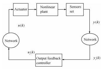 图 1 Framework of output feedback control systems over network environment.Fig. 1 Framework of output feedback control systems over network environment.
The sensors are connected to a network, which are shared by other NCSs and susceptible to communication delays and missing measurements or pack dropouts). As Fig. 1 depicts, pack dropouts from the controller to actuator can take place stochastically. The fuzzy systems with multiple stochastic communication delays and uncertain parameters can be read as follows:
Plant Rule $i$: If $\theta_{1}(k) $ is $ M_{i1}$, and $\theta_{2}(k)$ is $M_{i2}$, and, $\ldots$, and $\theta_{p}(k)$ is $M_{ip}$, then
$ \begin{align} x(k+1)=&\ A_i(k)x(k)+A_{di}\sum\limits_{m=1}^{h}\alpha_m(k)x(k-\tau_m(k))\notag\\ & +B_{1i}u(k)+D_{1i}v(k)\notag\\ \tilde{y}(k)=&\ C_ix(k)+D_{1i}v(k)\notag\\ z(k)=&\ C_{zi}(k)+B_{2i}u(k)+D_{3i}v(k)\notag\\ x(k)=&\ \phi(k)\quad\forall\, {k}\in \mathbb{Z}^{-}, ~\, i=1, \ldots, r \end{align} $
(1) where $M_{ij}$ is the fuzzy set, $r$ stands for the number of If-then rules, and $\theta(k)=[\theta_1(k), \theta_2(k), \ldots, \theta_{p}(k)]$ is the premise variable vector, which is independent of the input variable $u(k)$. $x(k)\in \mathbb{R}^n$ is the state vector, $u(k)\in \mathbb{R}^m$, $\tilde{y}$ $\in$ $\mathbb{R}^s$ is the process output, $z(k)\in \mathbb{R}^q$ is the controlled output, $v(k)\in \mathbb{R}^p$ presents a vector of exogenous inputs, which belongs to $l_2[0, \infty)$, $\tau_m(k)$ $(m=1, 2, \ldots, h)$ are the communication delays that vary with the stochastic variables $\alpha_m(k)$, and $\phi(k)$ $(\forall\, {k}\in \mathbb{Z}^{-})$ is the initial state.
The stochastic variables $\alpha_m(k)\in \mathbb{R}$ $(m=1, 2, \ldots, h)$ in (1) are assumed to satisfy mutually uncorrelated Bernoulli-distributed-white sequences described as follows:
$ \begin{align} & {\rm Prob}\{\alpha_m(k)=1\}={E}\{\alpha_m(k)\}=\bar{\alpha}_m\notag\\ & {\rm Prob}\{\alpha_m(k)=0\}=1-\bar{\alpha}_m.\notag \end{align} $
In this note, one can make the random communication-time delays satisfy the following assumption that the time-varying $\tau_m(k)$ $ (m=1, 2, \ldots, h)$ are subject to $ d_t\leq \tau_m(k)$ $\leq$ $d_T$. The matrices $A_i(k)=A_i+\Delta{A_i(k)}$, $C_{zi}(k)= C_{zi}$ $+$ $\Delta{C_{zi}}(k)$, where $ A_i, A_{di}, B_{1i}, B_{2i}, C_i, C_{zi}, D_{1i}, D_{2i}$, and $D_{3i}$ are known constant matrices with compatible dimensions. $\Delta{A_i(k)} $ and $\Delta C_{zi}(k)$ with the time-varying norm-bounded uncertainties satisfy
$ \begin{align} \left[ \begin{array}{c} \Delta A_i(k)\\ \Delta C_{zi}(k)\\ \end{array} \right]=\left[ \begin{array}{c} H_{ai}\\ H_{ci}\\ \end{array} \right]F(k)E \end{align} $
(2) with $H_{ai}$, $H_{ci}$ being constant matrices and $F^T(k)F(k)\leq I$, $\forall\, {k}$.
In this note, the packet dropout (the miss-measurement) read as
$ \begin{align} y_c(k)&= \Xi{C_i}x(k)+D_{2i}(k)\notag\\ &=\sum\limits_{l=1}^{s}\beta_lC_{il}x(k)+D_{2i}v(k)\notag\\ u(k)&=W(k)u_c(k)=W(k)C_{ki}x_c(k) \end{align} $
(3) where $\Xi=\hbox{diag}\{\beta_1, \ldots, \beta_s\}$ with $\beta_l$ $(l=1, 2, \ldots, s)$ being $s$ unrelated random variables, which are also unrelated with $\alpha_m(k)$ and $W(k)$ denoting the random packet missing from the controllers to the actuator. One can assume that $\beta_l $ has the probabilistic-density function $q_l(s)$ $(l=1, 2, \ldots, s)$ on the interval $[0, 1]$ with mathematical expectation $\mu_l$ and variance $\sigma_l^2$. $C_{il}={\rm diag}\{\underbrace{0, \ldots, 0}\limits_{l-1}, 1, \underbrace{0, \ldots, 0}\limits_{s-l}\}C_i$. We denote the stochastic pack dropouts from the controller to the actuator by $W(k)= {\rm diag}\{\omega_1(k), \ldots, \omega_m(k)\}$, where $\omega_l$ $(l=$ $1, 2, \ldots, m)$ are mutually unrelated random variables and obey Bernoulli distribution with mathematical expectation $\bar{\omega}_l$ and variance$\rho_l $and assumed to be unrelated with $\alpha_m(k)$. For a given pair of $(x(k), u(k))$, the final output of the fuzzy system is read as
$ \begin{align} x(k+1)=&\, \sum\limits_{i=1}^{r}h_i(\theta(k))[A_i(k)x(k)+B_{1, i}u(k)\notag\\ &\, +A_{di}\sum\limits_{m=1}^{h}x(k-\tau_m(k))+D_{1i}v(k)]\notag\\ y_c(k)=&\, \sum\limits_{i=1}^{r}h_i(\theta(k))[\Xi{C_i}x(k)+D_{2i}v(k)]\notag\\ z(k)=&\, \sum\limits_{i=1}^{r}h_i(\theta(k))[C_{zi}(k)x(k)+B_{2i}u(k)+D_{3i}v(k)] \end{align} $
(4) where the fuzzy-basis functions are described as
$ \begin{align} &{h_i(\theta(k))}=\frac {\vartheta_i(\theta(k))} {\sum\limits_{i=1}^{r}\vartheta_i(\theta(k))}\notag\\ &\vartheta_i(\theta(k))=\prod\limits_{j=1}^{p}M_{ij}(\theta_j(k))\notag \end{align} $
with $M_{ij}(\theta_j(k))$ being the grade of membership of $\theta_j(k)$ in $M_{ij}$. It is clear that $\vartheta_i(\theta(k))\geq 0$, $i=1, 2, \ldots, r$, $\sum_{i=1}^{r}\vartheta_i(\theta(k))>0$, $\forall\, {k}$, and $h_i(\theta(k))\geq 0$, $i=1, 2, \ldots, r$, $\sum_{i=1}^{r}h_i(\theta(k))=1$, $\forall\, {k}$. In the sequel, we denote $h_i=h_i(\theta(k))$ for brevity.
In the note, the fuzzy dynamic output-feedback controller for the fuzzy system (4) is given as
Controller Rule $i$: If $\theta_1(k)$ is $M_{il}$ and $\theta_2(k)$ is $M_{i2}$ and, $\ldots$, and $\theta_p(k)$ is $M_{ip}$ then
$ \begin{align} \begin{cases} x_c(k+1)=A_{ki}x_c(k)+B_{ki}y_c(k)\\ u(k)= W(k)C_{ki}x_c(k) \end{cases} \end{align} $
(5) with $x_c(k)\in \mathbb{R}^n$ being the controller state along with the controller parameters $A_{ki}$, $B_{ki}$ and $C_{ki}$ to be determined. Naturally, the overall fuzzy output-feedback controller is read as
$ \begin{align} \begin{cases} x_c(k+1)=\sum\limits_{i=1}^{r}h_i[A_{ki}x_c(k)+B_{ki}y(k)]\\ u(k)=\sum\limits_{i=1}^{r}h_iW(k)C_{ki}x_c(k), \ \ i=1, 2, \ldots, r. \end{cases} \end{align} $
(6) Combining (6) with (4), we can obtain the closed-loop system described as
$ \begin{align} \begin{cases} \bar{x}(k+1)=\sum\limits_{i-1}^{r}\sum\limits_{j=1}^{r}h_ih_j[(A_{ij}+B_{ij})\bar{x}(k)+D_{ij}v(k) \\ \qquad \qquad \quad\, +\sum\limits_{m=1}^{h}(\bar{A}_{dmi}+\tilde{A}_{dmi})\bar{x}(k-\tau_m(k)]\\ z(k)=\sum\limits_{i=1}^{r}\sum\limits_{j=1}^{r}h_ih_j[\bar{C}_{ij}(k)+\bar{\bar{C}}_{ij}]\bar{x}(k) +D_{3i}v(k) \end{cases} \end{align} $
(7) where
$ \begin{align*} &\bar{x}(k)=\left[ \begin{array}{c} x(k) \\ x_c(k) \\ \end{array} \right], \quad A_{ij}=\left[ \begin{array}{cc} A_i(k)&B_{1i}\bar{W}C_{kj} \\ B_{ki}\bar{\Xi}C_j&A_{ki} \\ \end{array} \right]\\[1mm] &B_{ij}=\left[ \begin{array}{cc} 0& B_{1i}\tilde{W}(k)C_{kj}\\ B_{ki}\tilde{\Xi}C_j& 0\\ \end{array} \right]\\[1mm] &\bar{A}_{dmi}=\left[ \begin{array}{cc} \bar{\alpha}_mA_{di}&0 \\ 0&0 \\ \end{array} \right], \quad \tilde{A}_{dmi}=\left[ \begin{array}{cc} \tilde{\alpha}_mA_{di}&0 \\ 0&0 \\ \end{array} \right]\\[1mm] &D_{ij}=\left[ \begin{array}{c} D_{1i} \\ B_{ki}D_{2j} \\ \end{array} \right], \quad \bar{C}_{ij}(k)=\bigg[ \begin{array}{cc} C_{zi}(k)&B_{2i}\bar{W}C_{kj} \\ \end{array} \bigg]\\[1mm] &\bar{\bar{C}}_{ij}(k)=\bigg[ \begin{array}{cc} 0&B_{2i}\tilde{W}(k)C_{kj} \\ \end{array} \bigg] \end{align*} $
with $\tilde{\alpha}_m(k)=\alpha_m(k)-\bar{\alpha}_m(k)$ and $\tilde{\omega}_j(k)={\omega}_j(k)-\bar{\omega}_j(k)$. It is evident that $E\{\tilde{\alpha}_m(k)\}=0$ and that $E\{\tilde{\omega}_j(k)\}=0$ and that $E\{\tilde{\alpha}_m^2(k)\}=\bar{\alpha}_m(1-\bar{\alpha}_m)=\sigma_m^2$ and that $E\{\tilde{\omega}_j^2(k)\}$ $=$ $\bar{\omega}_j(1-\bar{\omega}_j)=\rho_j^2$.
Denote
$ \begin{align*} &\bar{x}(k-\tau)\\ &=\left[ \!\!\begin{array}{cccc} \ \ \bar{x}^T(k-\tau_1(k)) &\!\bar{x}^T(k-\tau_2(k))&\! \cdots &\!\bar{x}^T(k-\tau_h(k))\ \ \\ \end{array} \!\!\right]^T\\ &\xi(k)=\left[ \begin{array}{ccc} \bar{x}^T(k)&\bar{x}^T(k-\tau) &v^T(k) \\ \end{array} \right]^T\end{align*} $
then (7) can also be rewritten as
$ \begin{align} \begin{cases} \bar{x}(k+1) =\sum\limits_{i=1}^{r}\sum\limits_{j=1}^{r}h_ih_j\left[A_{ij}\!+B_{ij}, \hat{Z}_{mi}\!+\Delta\hat{Z}_{mi}, D_{ij}\right]\xi(k) \\ z(k)=\sum\limits_{i=1}^{r}\sum\limits_{j=1}^{r}h_ih_j\left[\bar{C}_{ij}+ \bar{\bar{C}}_{ij}, 0, D_{3i}\right]\xi(k) \end{cases} \end{align} $
(8) where $\hat{Z}_{mi}=[\bar{A}_{d1i}, \ldots, \bar{A}_{dhi}]$ and $\Delta\hat{Z}_{mi}=[\tilde{A}_{d1i}, \ldots, \tilde{A}_{dhi}]$. In order to smoothly formulate the problem in the note, we introduce the following definition.
Definition 1: For the system (7) and every initial conditions $\phi$, the trivial solution is said to be exponentially mean square stable if, in the case of $v(k)=0$, there exist constants $\delta>0$ and $0<\kappa<1$ such that $E\{\|\bar{x}(k)\|^2\}$ $\leq$ $\delta\kappa^k \sup_{-d_M\leq i\leq 0}E\{\|{\phi(i)}\|^2\}$, $\forall\, {k}\geq 0$.
We will develop techniques to settle the robust $H_{\infty}$ dynamic output feedback problem for the discrete-time fuzzy system (7) subject to the following conditions:
1) The fuzzy system (7) is exponentially stable in the mean square.
2) Under zero-initial condition, the controlled output $z(k)$ satisfies
$ \begin{align} \sum\limits_{k=0}^{\infty}E\left\{\|{z(k)}\|^2\right\}\leq \gamma^2\sum\limits_{k=0}^{\infty}E\left\{\|{v(k)}\|^2\right\} \end{align} $
(9) for all nonzero $v(k)$, where $\gamma>0$ is a prescribed scalar.
Remark 1: The proposed new model has the function that not only the controllers communicate with the actuator by wireless but also the sensors do with the controllers by the same manner.
3. Development of Robust ${\pmb H}_{\pmb \infty}$ Fuzzy Control Performance
At first, we give the following lemma, which will be adopted in obtaining our main results.
Lemma 1 (Schur complement): Given constant matrices $S_1$, $S_2$, $S_3$, where $S_1=S_1^T$ and $0<S_2=S_2^T$, then $ S_1$ $+$ $S_3^TS_2^{-1}S_3$ $<$ $0$ if and only if
$ \begin{align*} \left[ \begin{array}{cc} S_1&S_3^T \\ S_3 &-S_2 \\ \end{array} \right]<0~~ \hbox{or}~~ \left[ \begin{array}{cc} -S_2&S_3 \\ S_3^T&S_1 \\ \end{array} \right]<0. \end{align*} $
Lemma 2 (S-procedure) [5]: Letting $L=L^T$ and $H$ and $E$ be real matrices of appropriate dimensions with $F$ satisfying $FF^T\leq I$, then $ L+HFE+E^TF^TH^T<0$ if and only if there exists a positive scalar $\varepsilon>0$ such that $L$ $+$ $\varepsilon^{-1}HH^T+\varepsilon E^TE<0$, or equivalently
$ \begin{align*} \left[ \begin{array}{ccc} L&H&\varepsilon{E^T} \\ H^T &-\varepsilon{I}&0 \\ \varepsilon{E}&0 &-\varepsilon{I} \\ \end{array} \right]<0. \end{align*} $
Lemma 3: For any real matrices $X_{ij}$ for $i$, $j=1, 2, \ldots, $ $r$ and $n>0$ with appropriate dimensions, we have [35]
$ \sum\limits_{i=1}^r\sum\limits_{j=1}^r\sum\limits_{l=1}^r\sum\limits_{l=1}^rh_ih_jh_kh_lX_{ij}^T\Lambda{X_{kl}}\leq\sum\limits_{i=1}^r\sum\limits_{j=1}^rh_ih_jX_{ij}^T\Lambda X_{ij}. $
Theorem 1: For given controller parameters and a prescribed $H_{\infty}$ performance $\gamma>0$, the nominal fuzzy system (7) is exponentially stable if there exist matrices $P>0$ and $Q_k$ $>$ $0$, $k=1, 2, \ldots, h$, satisfying
$ \left[ \begin{array}{cc} \Pi_i&\star \\ 0.5\Sigma_{ii}&\bigwedge \\ \end{array} \right]<0 $
(10) $ \left[ \begin{array}{cc} 4\Pi_i&\star \\ \Sigma_{ij}&\bigwedge \\ \end{array} \right]<0, \quad 1\leq i<j\leq r $
(11) where
$ \Pi_i =\ {\rm diag}\bigg\{-P+\sum\limits_{k=1}^h(d_T-d_t+1)Q_k, \hat{\alpha}\breve{A}_{di}^T\breve{P} \breve{A}_{di}\notag\\ \ \ \ \ \ \ -{\rm diag}\{Q_1, Q_2, \ldots, Q_h\}, -\gamma^2I\bigg\} $
(12) $\begin{align*} \hat{\alpha}=&\ {\rm diag}\left\{\bar{\alpha}_1(1-\bar{\alpha}_1), \ldots, \bar{\alpha}_h(1-\bar{\alpha}_h)\right\}\notag\\ \breve{A}_{di}=&\ {\rm diag}\{\underbrace{\hat{A}_{di}, \ldots, \hat{A}_{di}}\limits_h\}\notag\\ \check{C}_{ij}=&\ \left[\sigma_1\hat{C}_{11ij}^TP, \ldots\!, \sigma_s\hat{C}_{1sij}^TP, \rho_1\hat{C}_{k1ij}^TP, \ldots\!, \rho_m\hat{C}_{kmij}^TP\right]^T\notag\\ &\check{P}=\hbox{diag}\{\underbrace{P, \ldots, P}\limits_{s+m}\}\\ &{\small\bigwedge}=\hbox{diag}\{-\check{P}, -P, -I, \hbox{diag}\{\underbrace{-I, \ldots, -I}\limits_m\}\}\\ &\breve{P}=\hbox{diag}\{\underbrace{P, \ldots, P}\limits_h\}\\ &\hat{A}_{di}=\left[ \begin{array}{cc} A_{di}&0\\ 0&0\\ \end{array} \right] \\ &\Sigma_{ij}=\\ &\!\!\!\left[\!\!{\small \begin{array}{ccccc} \check{C}_{ij}\!+\!\check{C}_{ji}\! &\! 0\!&\!0 \\[2mm] PA_{ij}\!+\!PA_{ji} \! &\! P\hat{Z}_{mi}\!+\!P\hat{Z}_{mj} \! &\!PD_{ij}\!+\!PD_{ji}\\[2mm] \bar{C}_{ij}\!+\!\bar{C}_{ji}\! &\!0\! &\!D_{3i}\!+\!D_{3j}\\[2mm] \, [0 ~~ \rho_1B_{2i}C_{kj1}\!+\!\rho_1B_{2j}C_{ki1}] \! &\!0\! &\!0\\[2mm] \vdots\! &\!\vdots\! &\!\vdots\\[2mm] \, [0 ~~ \rho_mB_{2i}C_{kjm}\!+\!\rho_mB_{2j}C_{kim}]\! &\!0\! &\!0\\ \end{array}}\!\!\!\! \right]. \end{align*} $
Proof:
Let
$ \begin{align*} &\Theta_j(k)=\{x(k-\tau_j(k), x(k-\tau_j(k)+1, \ldots, x(k)\}\\ &\chi(k)=\{\Theta_1(k)\bigcup\Theta_2(k)\bigcup\ldots\bigcup\Theta_h(k)\}=\bigcup\limits_{j=1}^{h}\Theta_j(k) \end{align*} $
where $j=1, 2, \ldots, h$. We consider the following Lyapunov functional for the system of (7): $V(\chi(k))=\sum_{i=1}^3V_i(k)$, where
$ \begin{align*} &V_1(k)=\bar{x}^T(k)P\bar{x}\\ &V_2(k)=\sum\limits_{j=1}^{h}\sum\limits_{i=k-\tau_j(k)}^{k-1}\bar{x}^T(i)Q_j\bar{x}(i)\\ &V_3(k)=\sum\limits_{j=1}^h\sum\limits_{m=-d_M+1}^{-d_m}\sum\limits_{i=k+m}^{k-1}\bar{x}^T(i)Q_j\bar{x}(i) \end{align*} $
with $P>0$, $Q_j>0$ $(j=1, 2, \ldots, h)$ being matrices to be determined.
$ \begin{align} {E}[\Delta{V}|x(k)]&={E}[V(\chi(k+1))|\chi(k)]-V(\chi(k))\notag\\ & ={E}[(V(\chi(k+1))-V(\chi(k)))|\chi(k)]\notag\\ & =\sum\limits_{i=1}^{3}{E}[\Delta{V_i}|\chi(k)]. \end{align} $
(13) According to (7), we have
$ \begin{align*} &{E}\{\Delta{V_1}|\chi(k)\}\\ &\qquad={E} \left[(\bar{x}^T(k+1)P\bar{x}(k+1)-\bar{x}^T(k)P\bar{x}(k))|\chi(k)\right]\\ &\qquad\leq\xi^T(k)\sum\limits_{i=1}^{r}\sum\limits_{j=1}^{r}\Omega_{ij}\xi(k) \end{align*} $
where
$ \begin{align} & {{\Omega }_{ij}}=E\left\{ \left[\begin{matrix} A_{ij}^{T}P{{A}_{ij}}+B_{ij}^{T}P{{B}_{ij}}-P & {} \\ \star & {} \\ \star & {} \\ \end{matrix} \right. \right. \\ & \left. \left. \begin{matrix} {} & A_{ij}^{T}P{{{\hat{Z}}}_{mi}} & A_{ij}^{T}P{{D}_{ij}} \\ {} & \hat{Z}_{mi}^{T}P{{{\hat{Z}}}_{mi}}+\Delta \hat{Z}_{mi}^{T}P\Delta {{{\hat{Z}}}_{mi}} & \hat{Z}_{mi}^{T}P{{D}_{ij}} \\ {} & \star & D_{ij}^{T}P{{D}_{ij}} \\ \end{matrix} \right] \right\} \\ \end{align} $
$ {{B}_{ij}}=\left[\begin{matrix} 0 & 0 \\ {{B}_{ki}}\tilde{\Xi }{{C}_{j}} & 0 \\ \end{matrix} \right]+\left[\begin{matrix} 0 & {{B}_{1i}}\tilde{\omega }(k){{C}_{kj}} \\ 0 & 0 \\ \end{matrix} \right] $
$ \begin{align} & E\{B_{ij}^{T}P{{B}_{ij}}\} \\ & \ \ \ \ \ =\sum\limits_{l=1}^{s}{\sigma _{l}^{2}}{{\left[\begin{matrix} 0 & 0 \\ {{B}_{ki}}{{C}_{jl}} & 0 \\ \end{matrix} \right]}^{T}}P\left[\begin{matrix} 0 & 0 \\ {{B}_{ki}}{{C}_{jl}} & 0 \\ \end{matrix} \right] \\ & \ \ \ \ \ +\sum\limits_{l=1}^{m}{\rho _{l}^{2}}{{\left[\begin{matrix} 0 & {{B}_{1i}}{{C}_{kjl}} \\ 0 & 0 \\ \end{matrix} \right]}^{T}}P\left[\begin{matrix} 0 & {{B}_{1i}}{{C}_{kjl}} \\ 0 & 0 \\ \end{matrix} \right] \\ & \ \ \ ={{({{{\overset{\lower0.5em\hbox{$\smash{\scriptscriptstyle\smile}$}}{P}}}^{-1}}{{{\overset{\lower0.5em\hbox{$\smash{\scriptscriptstyle\smile}$}}{C}}}_{lij}})}^{T}}\overset{\lower0.5em\hbox{$\smash{\scriptscriptstyle\smile}$}}{P}({{{\overset{\lower0.5em\hbox{$\smash{\scriptscriptstyle\smile}$}}{P}}}^{-1}}{{{\overset{\lower0.5em\hbox{$\smash{\scriptscriptstyle\smile}$}}{C}}}_{lij}}) \\ \end{align} $
$ \begin{align} & \overset{\lower0.5em\hbox{$\smash{\scriptscriptstyle\smile}$}}{P}=\rm{diag}\{\underbrace{\mathit{P}, \ldots, \mathit{P}}_{\mathit{s}+\mathit{m}}\} \\ & {{{\hat{C}}}_{1lij}}=\left[\begin{matrix} 0 & 0 \\ {{B}_{ki}}{{C}_{jl}} & 0 \\ \end{matrix} \right] \\ & {{{\hat{C}}}_{klij}}=\left[\begin{matrix} 0 & {{B}_{1i}}{{C}_{kjl}} \\ 0 & 0 \\ \end{matrix} \right] \\ & {{{\overset{\lower0.5em\hbox{$\smash{\scriptscriptstyle\smile}$}}{C}}}_{ij}}={{\left[{{\sigma }_{1}}\hat{C}_{11ij}^{T}P, \ldots, {{\sigma }_{s}}\hat{C}_{1sij}^{T}P, {{\rho }_{1}}\hat{C}_{k1ij}^{T}P, \ldots, {{\rho }_{m}}\hat{C}_{kmij}^{T}P \right]}^{T}} \\ \end{align} $
$ \begin{align} & E\left\{ \Delta \hat{Z}_{mi}^{T}P\Delta {{{\hat{Z}}}_{mi}} \right\} \\ & \ \ \ \ \ =\sum\limits_{m=1}^{h}{{{{\bar{\alpha }}}_{m}}}(1-{{{\bar{\alpha }}}_{m}}){{\left[ \begin{matrix} {{A}_{di}} & 0 \\ 0 & 0 \\ \end{matrix} \right]}^{T}}P\left[ \begin{matrix} {{A}_{di}} & 0 \\ 0 & 0 \\ \end{matrix} \right] \\ & \ \ \ \ \ \ =\sum\limits_{m=1}^{h}{\hat{A}_{di}^{T}}P{{{\hat{A}}}_{di}}=\hat{\alpha }\overset{\lower0.5em\hbox{$\smash{\scriptscriptstyle\smile}$}}{A}_{di}^{T}\overset{\lower0.5em\hbox{$\smash{\scriptscriptstyle\smile}$}}{P}{{{\overset{\lower0.5em\hbox{$\smash{\scriptscriptstyle\smile}$}}{A}}}_{di}} \\ \end{align} $
$ \begin{align} & \hat{\alpha }=\rm{diag}\{{{{\bar{\alpha }}}_{1}}(1-{{{\bar{\alpha }}}_{1}}), \ldots, {{{\bar{\alpha }}}_\mathit{h}}(1-{{{\bar{\alpha }}}_\mathit{h}})\} \\ & {{{\overset{\lower0.5em\hbox{$\smash{\scriptscriptstyle\smile}$}}{A}}}_{di}}=\rm{diag}\{\underbrace{\mathit{{{\hat{A}}}_{di}}, \ldots, \mathit{{{\hat{A}}}_{di}}}_\mathit{h}\} \\ & E\{\Delta {{V}_{2}}|\chi (k)\}\le E\{\sum\limits_{j=1}^{h}{({{{\bar{x}}}^{T}}(}k){{Q}_{j}}\bar{x}(k) \\ & \ \ \ \ \ -{{{\bar{x}}}^{T}}(k-{{\tau }_{j}}(k)){{Q}_{j}}\bar{x}(k-{{\tau }_{j}}(k)) \\ & \ \ \ \ \ +\sum\limits_{i=k-{{d}_{M}}+1}^{k-{{d}_{m}}}{{{{\bar{x}}}^{T}}}(i){{Q}_{j}}\bar{x}(i))|\chi (k)\} \\ & E\{\Delta {{V}_{3}}|\chi (k)\}=E\{\sum\limits_{j=1}^{h}{((}{{d}_{T}}-{{d}_{t}}){{{\bar{x}}}^{T}}(k){{Q}_{j}}\bar{x}(k) \\ & \ \ \ \ \ -\sum\limits_{i=k-{{d}_{m}}+1}^{k-{{d}_{m}}}{{{{\bar{x}}}^{T}}}(i){{Q}_{j}}\bar{x}(i))|\chi (k)\}. \\ \end{align} $
It is clear that
$ {E}\{\Delta{V_2}|\chi(k)\}+{E}\{\Delta{V_3}|\chi(k)\}\leq\xi^T(k)T_{ij}\xi(k) $
with
$ \begin{align*} T_{ij}=&\ \hbox{diag}\Bigg\{\sum\limits_{k=1}^h(d_T-d_t+1)Q_k, \\ &-\hbox{diag}\{Q_1, Q_2, \ldots, Q_h\}, 0\Bigg\}.\end{align*} $
Therefore, we have ${E}\{\Delta{V}|\chi(k)\}\leq\xi^T(k)\Gamma_{ij}\xi(k)$, where $\Gamma_{ij}$ $=$ $\Omega_{ij}+T_{ij}$. Due to
$ \begin{align*} &{E}\left\{z^T(k)z(k)-\gamma^2v^T(k)v(k)\right\}\\ &\qquad\leq\xi(k)\sum\limits_{i=1}^r\sum\limits_{j=1}^rh_ih_j {E}\left\{[\bar{C}_{ij}+\bar{\bar{C}}_{ij}, 0, D_{3i}]^T\right.\\ &\qquad\quad \left.\times[\bar{C}_{ij}+\bar{\bar{C}}_{ij}, 0, D_{3i}] - \hbox{diag}\{0, 0, \gamma^2I\}\right\}\xi(k) \end{align*} $
we can obtain
$ \begin{align*} &{E}\left\{z^T(k)z(k)-\gamma^2v^T(k)v(k)+\Delta{V(k)}\right\}\\ &\qquad \leq\xi^T(k)({\Omega}_{ij}^T\hbox{diag} \{P, I\}{\Omega}_{ij}\\ &\qquad\quad +\mathcal{Z}_{ij}^T\hbox{diag}\{\check{P}, I\}\mathcal{Z}_{ij}+\bar{P})\xi(k) \end{align*} $
where
$ \begin{align*} &{\Omega}_{ij}=\left[ \begin{array}{ccc} A_{ij}&\hat{Z}_{mi}&D_{ij}\\ \bar{C}_{ij}&0&D_{3i}\\ \end{array} \right]\\ & \Game _{kijt}= \bigg[ \begin{array}{ccc} \left[ \begin{array}{cc} 0&\rho_tB_{2i}C_{kjt} \end{array} \right]&0&0 \end{array} \bigg]^T \\ &\mathfrak{D}_{ij}=\bigg[ \begin{array}{ccc} \Game_{kij1}&\ldots&\Game_{kijm} \end{array} \bigg]^T \\ &\mathcal{Z}_{ij}=\left[ \begin{array}{c} [\check{P}^{-1}\check{C}_{ij}, 0, 0]\\ \mathfrak{D}_{ij} \end{array} \right]\\ &\bar{P}=\hbox{diag}\bigg\{-P+\sum\limits_{k=1}^h(d_T-d_t+1)Q_k, \hat{\alpha}\breve{A}_{di}^T\breve{P} \breve{A}_{di}\\ &\qquad -\hbox{diag}\{Q_1, Q_2, \ldots, Q_h\}, -\gamma^2I\bigg\}. \end{align*} $
Define $J(n)={E}\sum\nolimits_{k=0}^n[z^T(k)z(k)-\gamma^2v^T(k)v(k)]$, we have
$ \begin{align*} J(n)=&\ {E}\sum\limits_{k=0}^n\left[z^T(k)z(k)-\gamma^2v^T(k)v(k)+\Delta{V(\chi(k))}\right] \\ &-{E}V(\chi(n+1))\\ \leq&\ {E}\sum\limits_{k=0}^n\left[z^T(k)z(k)-\gamma^2v^T(k)v(k)+\Delta{V(\chi(k))}\right]\\ \leq&\ \sum\limits_{k=0}^n\sum\limits_{i=1}^r\sum\limits_{j=1}^rh_ih_j\xi^T(k)({\Omega}_{ij}^T \hbox{diag} \{P, I\}{\Omega}_{ij}\\ &\ +\mathcal{Z}_{ij}^T\hbox{diag}\{\check{P}, I\}\mathcal{Z}_{ij}+\bar{P})\xi(k)\\ =&\ \sum\limits_{k=0}^n\sum\limits_{i=1}^rh_i^2\xi^T(k)({\Omega}_{ii}^T \hbox{diag} \{P, I\}{\Omega}_{ii}\\ &\ +\mathcal{Z}_{ii}^T\hbox{diag}\{\check{P}, I\}\mathcal{Z}_{ii}+\bar{P})\xi(k)\\ &\ +\frac{1}{2}\sum\limits_{k=0}^n\sum\limits_{j=1, i<j}^rh_ih_j\xi^T(k)\\ &\ \times\left[({\Omega}_{ij} +{\Omega}_{ji})^T\hbox{diag}\{P, I\}({\Omega}_{ij}+{\Omega}_{ji})\right.\\ &\ +\left. (\mathcal{Z}_{ij}+\mathcal{Z}_{ji})^T\hbox{diag}\{\check{P}, I\} (\mathcal{Z}_{ij}+\mathcal{Z}_{ji})+4\bar{P}\right]\xi(k). \end{align*} $
According to Schur complement, we can conclude from (10) and (11) that $J(n)<0$. Letting $n\rightarrow\infty$, we have
$ \begin{align*} \sum\limits_n^\infty{E}\left\{\|z(k)\|^2\right\}\leq\gamma^2\sum\limits_n^\infty{E}\left\{\|v(k)\|^2\right\}. \end{align*} $
According to Schur complement again, we know that ${E}\{\Delta{V}|x(k)\}$ $<$ $0$ if and only if (10) and (11) hold true. Furthermore, one can easily verify the fact that the discrete-time nominal (7) with $v(k)=0$ is exponentially stable.
4. Design of Robust ${\pmb H}_{\pmb\infty}$ Fuzzy Controller
In this section, we are devoted to how to determine the controller parameters in (6) such that the closed-loop system (7) is exponentially stable with $H_\infty$ performace.
By Theorem 1, one can easily draw the conclusion as follow:
Theorem 2: For a prescribed constant $\gamma>0$, the nominal fuzzy system (7) is exponentially stable if there exist positive definite matrices $P>0$, $L>0$, $Q_k>0$ $(k=1, 2, $ $\ldots, $ $h)$, and $K_i$ and $\bar{C}_{ki}$ such that
$ \Gamma_1=\left[ \begin{array}{cc} \Pi_i&\star \\ 0.5\bar{\Sigma}_{ii}& \bar{\Lambda} \\ \end{array} \right]<0, \ \ i=1, 2, \ldots, r $
(14) $ \Gamma_2=\left[ \begin{array}{cc} 4\Pi_i&\star \\ \bar{\Sigma}_{ij}&\bar{\Lambda} \\ \end{array} \right]<0, \ \ 1\leq i<j\leq r $
(15) $ PL=I $
(16) hold, then the nominal system (7) is exponentially stable with disturbance attenuation $\gamma$, where $\overline{\bigwedge}=\hbox{diag}\{-\bar{L}, -L, $ $-I, $ $\hbox{diag}\{\underbrace{-I, \ldots, -I}\limits_m\}\}$
$ \bar{\Sigma}_{ij}=\left[ \begin{array}{ccc} \Phi_{11ij}+\Phi_{11ji}&0&0 \\ \Phi_{21ij}+\Phi_{21ji}&\Phi_{22ij}+\Phi_{22ji}& \Phi_{23ij}+\Phi_{23ji} \\ \Phi_{31ij}+\Phi_{31ji}&0&\Phi_{33ij}+\Phi_{33ji} \\ \Phi_{41ij}+\Phi_{41ji}&0&0 \\ \end{array} \right] $
(17) $\begin{align} &I_l=\hbox{diag}\{\underbrace{0, \ldots, 0}\limits_{l-1}, 1, \underbrace{0, \ldots, 0}\limits_{m-l}\}, \quad K_i=\bigg[ \begin{array}{cc} A_{ki}&B_{ki}\\ \end{array}\bigg] \notag\\[1mm] &\bar{C}_{ki}=\bigg[ \begin{array}{cc} 0&C_{ki}\\ \end{array} \bigg], \quad \bar{E}=\left[ \begin{array}{c} 0 \\ I \\ \end{array} \right], \quad \bar{\bar{E}}=\left[ \begin{array}{l} I \\ 0 \\ \end{array} \right] \notag\\[1mm] &\bar{A}_i=\left[ \begin{array}{cc} A_i&0 \\ 0&0 \\ \end{array} \right], \quad \bar{B}_{1i}=\left[ \begin{array}{c} B_{1i} \\ 0 \\ \end{array} \right], \quad R_{il}=\left[ \begin{array}{cc} 0&0 \\ C_{il}&0 \\ \end{array} \right] \notag\\[1mm] &\bar{D}_{1i}=\left[ \begin{array}{c} D_{1i} \\ 0 \\ \end{array} \right], \quad \bar{D}_{2i}=\left[ \begin{array}{c} 0 \\ D_{2i} \\ \end{array} \right]\notag\\[1mm] & \Phi_{11ij}=\left[ \begin{array}{c} \sigma_1\bar{E}K_iR_{j1} \\ \vdots \\ \sigma_s\bar{E}K_iR_{js} \\ \rho_1\bar{E}\beta_{1i}I_1\bar{C}_{kj} \\ \vdots \\ \rho_m\bar{E}\beta_{1i}I_m\bar{C}_{kj} \\ \end{array} \right], \ \ \Phi_{41ij}=\left[ \begin{array}{c} \rho_1B_{2i}I_1\bar{C}_{kj} \\ \vdots \\ \rho_mB_{2i}I_m\bar{C}_{kj} \\ \end{array} \right]\notag\\[1mm] & \Phi_{21ij}=\bar{A}_i+\bar{E}K_i\bar{R}_j+\bar{B}_{1i}\hbox{diag}\{w_1, \ldots, w_m\}\bar{C} _{kj} \notag\\[1mm] &\Phi_{31ij}=\bar{C}_{zi}+B_{2i}\hbox{diag}\{w_1, \ldots, w_m\}\bar{C}_{kj}\notag \\[1mm] & \bar{C}_{zi}=\left[ \begin{array}{cc} C_{zi}&0 \\ \end{array} \right], \quad \bar{L}=\hbox{diag}\{\underbrace{L, \ldots, L} \limits_{s+m}\}\notag \\[1mm] & \Phi_{22ij}=\hat{Z}_{mi}, \quad \Phi_{23ij}=D_{ij}, \quad \Phi_{33ij}=D_{3i}.\notag \end{align} $
Proof: We rewrite the parameters in Theorem 1 in the following form:
$ \begin{align*} & A_{ij}=\bar{A}_i+\bar{E}K_i\bar{R}_j+\bar{B}_{1i}\hbox{diag}\{w_1, \ldots, w_m\}\bar{C}_{kj} \\ &\hat{C}_{lij}=\bar{E}K_i{R}_{jl} \\ & \bar{C}_{ij}=\bar{C}_{zi}+B_{2i}\hbox{diag}\{w_1, \ldots, w_m\}\bar{C}_{kj} \\ & D_{ij}=\bar{D}_{1i}+\bar{D}_{1i}K_i\bar{D}_{2j}. \end{align*} $
Pre-and post-multiplying the (10) and (11) by $ \hbox{diag}\{I, $ $I, $ $I, $ $\check{P}^{-1}, $ $P^{-1}, $ $\underbrace{I, \ldots, I}\limits_m\}$ and Letting $L=P^{-1}$, we have (14)$-$(16) and complete the proof easily. Now we will point out that the robust $H_\infty$ controller parameters can be determined in light of Theorem 2.
Theorem 3: For given scalar $\gamma>0$, if there exist positive define matrices $P>0$, $L>0$, $Q_k>0$ $(k=1, 2, \ldots, h)$, and matrices $K_i$, $\bar{C}_{ki}$ of proper dimensions and a constant $\varepsilon>0$ such that
$ \left[ \begin{array}{cc} \Gamma_1&\star \\ \Xi_{ii}&\hbox{diag}\{-\varepsilon{I}, -\varepsilon{I}\} \\ \end{array} \right]<0, \notag\\ \qquad\qquad\qquad\qquad\qquad i=1, 2, \ldots, r $
(18) $ \left[ \begin{array}{cc} \Gamma_2& \star \\ \Xi_{ij}&\hbox{diag}\{-\varepsilon{I}, -\varepsilon{I}\} \\ \end{array} \right]<0, \notag\\ \qquad\qquad\qquad\qquad\qquad 1\leq i<j\leq r $
(19) $ PL=I $
(20) hold, where
$ \begin{align*}&\Xi_{ii}=\left[ \begin{array}{ccccccc} 0&0&0&0&[H_{ai}^T ~~ 0] &H_{ci}^T&0 \\ \varepsilon[ E ~~ 0] &0&0&0&0&0&0 \\ \end{array} \right]\\ &\Xi_{ij}=\left[ \begin{array}{ccccccc} 0&0&0&0&[H_{ai}^T+H_{aj}^T ~~ 0] &H_{ci}^T+H_{cj}^T&0 \\ \varepsilon[E ~~ 0] &0&0&0&0&0&0 \\ \end{array} \right] \end{align*} $
then the uncertain fuzzy system (7) is exponentially stable and the controller parameters $K_i$ and $\bar{C}_{ki} $ can be obtained naturally.
Proof: Replace $\bar{A}_i$, $\bar{A}_j$, $\bar{C}_{zi}, $ and $ \bar{C}_{zj}$ in Theorem 2 by $\bar{A}_i+\triangle\bar{A}_i(k)$, $\bar{A}_j\triangle\bar{A}_j(k)$, $\bar{C}_{zi}+\triangle\bar{C}_{zi}(k), $ and $ \bar{C}_{zj}\, +\, \triangle\bar{C}_{zj}(k)$, respectively, where
$ \begin{align} & \triangle\bar{A}_i(k)=\left[ \begin{array}{cc} \triangle{A}_i(k)&0 \\ 0&0 \\ \end{array} \right], \quad \triangle\bar{C}_{zi}(k)=[ \triangle{C}_{zi}(k) ~~ 0].\!\notag \end{align} $
According to Lemma 1, (18) and (19) can be rewritten as follows:
$ \begin{align} &\Gamma_1+{H}_1F(k){E}+{E}^TF(k)^T{H}_1^T<0\notag\\ &\Gamma_2+{H}_2F(k){E}+{E}^TF(k)^T{H}_2^T<0\notag \end{align} $
where
$ \begin{align*} &{E}=[E ~~ 0]\\ &{H}_1=\left[ \begin{array}{ccccccc} 0& 0&0&0&[H_{ai}^T ~~ 0] &H_{ci}^T&0 \\ \end{array} \right]\\ & {H}_2=\left[ \begin{array}{ccccccc} 0& 0&0&0 &[H_{ai}^T+H_{aj}^T ~~ 0] &H_{ci}^T+H_{cj}^T&0 \\ \end{array} \right]. \end{align*} $
According to Lemma 1 along with Schur complement, we can easily obtain (18) and (19).
In order to solve (18), (19) and (20), the cone-complementarity linearization (CCL) algorithm proposed in [36] and [37] is used in this note.
The nonlinear minimization problem: $\min\hbox{tr}(PL) $ subject to (18) and (19) and
$ \left[ \begin{matrix} P & I \\ I & L \\ \end{matrix} \right]\ge 0. $
(21) The following algorithm [5] is borrowed to solve the above problem.
Algorithm 1:
Step 1: Find a feasible set $(P_0, L_0, Q_{k(0)}, K_{i(0)}, \bar{C}_{ki(0)})$ satisfying (18), (19) and (21). Set $q=0$.
Step 2: Solving the linear matrix inequality (LMI) problem, $\min\hbox{tr}(PL_{(0)}+P_{(0)}L) $ subject to (18), (19) and (21).
Step 3: Substitute the obtained matrix variables $(P$, $L$, $Q_{k}, K_{i(0)}, \bar{C}_{ki})$ into (14) and (15). If conditions(14) and (15) are satisfied with $|\hbox{tr}(PL)-n|<\delta$ for some sufficiently small scalar $\delta >0$, then output the feasible solutions. Exit.
Step 4: If $q>N$, where $N$ is the maximum number of iterations allowed, then output the feasible solutions $(P$, $L$, $Q_{k}, K_{i}$, $\bar{C}_{ki})$, and exit. Else, set $q=q+1$, and goto Step 2.
5. An Illustrative Example
we give an illustrative examples to explain the proposed model is effective and feasible in this section.
Example 1: Consider a T-S fuzzy model (1). The rules are given as follows:
Plant Rule 1: If $x_1(k)$ is $h_1(x_1(k))$ then
$ \begin{align} \begin{cases} x(k+1) = A_1(k)x(k)+A_{d1}\sum\limits_{m=1}^h\alpha_m(k)x(k-\tau_m(k))\\ \qquad\qquad\quad +~B_{11}u(k)+D_{11}v(k) \\[2mm] y(k) = \Xi C_1x(k) +D_{21}v(k) \\[2mm] z(k) = C_{z1}(k)x(k)+B_{21}u(k)+D_{31}v(k) \end{cases} \end{align} $
(21) Plant Rule 2: If $x_1(k)$ is $h_2(x_1(k))$ then
$ \begin{align} \begin{cases} x(k+1) = A_2(k)x(k)+A_{d2}\sum\limits_{m=1}^h\alpha_m(k)x(k-\tau_m(k))\\ \qquad\qquad\quad +~B_{12}u(k)+D_{12}v(k) \\[2mm] y(k) =\Xi C_2x(k) +D_{22}v(k) \\[2mm] z(k) =C_{z2}(k)x(k)+B_{22}u(k)+D_{32}v(k) \end{cases} \end{align} $
(22) The given model parameters are written as follows:
$ \begin{align} & {{A}_{1}}=\left[ \begin{matrix} 1 & 0.2 & 0 \\ 0.1 & 0.1 & 0.1 \\ 0.1 & 0.2 & 0.2 \\ \end{matrix} \right],\quad {{D}_{11}}=\left[ \begin{matrix} 0.1 \\ 0 \\ 0 \\ \end{matrix} \right] \\ & {{A}_{d1}}=\left[ \begin{matrix} 0.03 & 0 & -0.01 \\ 0.02 & 0.03 & 0 \\ 0.04 & 0.05 & -0.1 \\ \end{matrix} \right], \quad {{B}_{11}}=\left[ \begin{matrix} 1 & 1 \\ 0.4 & 1 \\ 0 & 1 \\ \end{matrix} \right] \\ & {{D}_{31}}=\left[ \begin{matrix} -0.1 \\ 0 \\ 0.1 \\ \end{matrix} \right], \quad \ {{C}_{1}}=\left[ \begin{matrix} 1 & 0.8 & 0.7 \\ -0.6 & 0.9 & 0.6 \\ \end{matrix} \right] \\ & {{C}_{2}}=\left[ \begin{matrix} 0.1 & 0.8 & 0.7 \\ -0.6 & 0.9 & 0.6 \\ \end{matrix} \right],\quad {{D}_{21}}=\left[ \begin{matrix} 0.15 \\ 0 \\ \end{matrix} \right] \\ & {{D}_{22}}=\left[ \begin{matrix} 0.1 \\ 0 \\ \end{matrix} \right], \quad \ {{C}_{z1}}=\left[ \begin{matrix} 0.2 & 0 & 0 \\ 0 & 0 & 0 \\ 0 & 0 & 0.1 \\ \end{matrix} \right] \\ & {{B}_{21}}=\left[ \begin{matrix} 1 & 1 \\ 0 & 1 \\ 0 & 1 \\ \end{matrix} \right], \quad {{H}_{a1}}=\left[ \begin{matrix} 0.1 \\ 0.1 \\ 0.1 \\ \end{matrix} \right],\quad {{H}_{c1}}=\left[ \begin{matrix} 0.1 \\ 0 \\ 0.1 \\ \end{matrix} \right] \\ & {{H}_{a2}}=\left[ \begin{matrix} 0.1 \\ 0 \\ 0.1 \\ \end{matrix} \right], \quad \ {{H}_{c2}}=\left[ \begin{matrix} 0.1 \\ 0 \\ 0.5 \\ \end{matrix} \right],\quad {{D}_{32}}=\left[ \begin{matrix} 0.1 \\ 0 \\ 0.1 \\ \end{matrix} \right] \\ & E={{\left[ \begin{matrix} 0.1 \\ 0.1 \\ 0.1 \\ \end{matrix} \right]}^{T}},{{A}_{2}}=\left[ \begin{matrix} 1 & -0.38 & 0 \\ -0.2 & 0 & 0.21 \\ 0.1 & 0 & -0.55 \\ \end{matrix} \right] \\ & {{B}_{12}}=\left[ \begin{matrix} 1 & 0 \\ 1 & 1 \\ 0 & 1 \\ \end{matrix} \right],\quad {{A}_{d2}}=\left[ \begin{matrix} 0 & 0.01 & -0.01 \\ 0.02 & 0.03 & 0 \\ 0.04 & 0.05 & -0.1 \\ \end{matrix} \right] \\ & {{D}_{12}}=\left[ \begin{matrix} 0.1 \\ 0 \\ 0.1 \\ \end{matrix} \right],\quad {{C}_{z2}}=\left[ \begin{matrix} 0.1 & 0 & 0 \\ 0.2 & 0 & 0.2 \\ 0 & 0.1 & 0.2 \\ \end{matrix} \right] \\ & {{B}_{22}}=\left[ \begin{matrix} 1 & 0 \\ 0 & 1 \\ 1 & 1 \\ \end{matrix} \right]. \\ \end{align} $
Assume that the time-varying communication delays satisfy $2 \leq\tau_m\leq 6$ $(m=1, 2)$ and
$ \begin{align*} & \bar{\alpha}_1={E}\{\alpha_1(k)\}=0.8, \quad\bar{\alpha}_2={E}\{\alpha_2(k)\}=0.6 \\[1mm] & \bar{\omega}_1={E}\{\omega_1(k)\}=0.4, \quad \bar{\omega}_2={E}\{\omega_2(k)\}=0.6. \end{align*} $
Assume also that the probabilistic density functions of $\beta_1$ and $\beta_2$ in $[0 \quad 1]$ are read as
$ \begin{align} q_1(s_1)=\begin{cases} 0,&s_1=0 \\ 0.1,&s_2=0.5 \\ 0.9,&s_3=1 \end{cases}, \quad &q_2(s_2)=\begin{cases} 0,& s_2=0\\ 0.2,&s_2=0.5 \\ 0.8,&s_3=1 \end{cases}. \end{align} $
(23) The membership functions are described as
$ \begin{align} &h_1=\begin{cases} 1,&x_0(1)=0 \\ \left|\dfrac{\sin(x_0(1))}{x_0(1)}\right|,&\hbox{else} \end{cases} \nonumber\\& h_2=1-h_1. \end{align} $
(24) Now, we are to design a dynamic-output feedback paralleled controller in the form of (6) such that (7) is exponentially stable with a given $H_\infty$ norm bound $\gamma$. In the example, we assume $\gamma=0.9$ and obtain the desired $H_\infty$ controller parameters as follows
$ \begin{align} & {{A}_{k1}}=\left[ \begin{matrix} -0.0127 & -0.0083 & -0.0317 \\ 0.0229 & 0.0149 & 0.0221 \\ -0.0588 & -0.0429 & -0.0654 \\ \end{matrix} \right] \\ & {{A}_{k2}}=\left[ \begin{matrix} -0.1365 & -0.1296 & -0.0570 \\ -0.0107 & -0.0095 & 0.0239 \\ -0.0125 & -0.0129 & -0.0260 \\ \end{matrix} \right] \\ & {{B}_{k1}}=\left[ \begin{matrix} -0.3236 & 0.1389 \\ 0.0291 & -0.0043 \\ -0.3077 & 0.1867 \\ \end{matrix} \right] \\ & {{B}_{k2}}=\left[ \begin{matrix} 0.1664 & 0.0834 \\ 0.1374 & -0.0712 \\ -0.4340 & 0.5688 \\ \end{matrix} \right] \\ & {{C}_{k1}}=\left[ \begin{matrix} 0.1355 & 0.0856 & 0.1789 \\ 0.0311 & 0.0209 & 0.0372 \\ \end{matrix} \right] \\ & {{C}_{k2}}=\left[ \begin{matrix} 0.0110 & 0.0464 & 0.0731 \\ 0.0832 & 0.0622 & 0.0502 \\ \end{matrix} \right]. \\ \end{align} $
We take the initial conditions $ x_0=[1 \quad 0 \quad-1]^T$, $x_{c0}$ $=$ $[0 \quad 0 \quad 0]^T $ for the simulation purpose and let external disturbance $v(k)=0$. Fig. 2 depicts the state responses for the uncontrolled fuzzy systems, which are unstable. We can see the fact that the closed-loop fuzzy systems are exponentially stable from the Fig. 3.
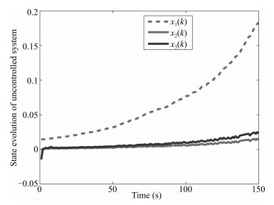 图 2 State evolution $x(k)$ of uncontrolled systems.Fig. 2 State evolution $x(k)$ of uncontrolled systems.
 图 3 State evolution $x(k)$ of controlled systems.Fig. 3 State evolution $x(k)$ of controlled systems.
In order to illustrate the disturbance-attenuation performance, we take the external disturbance
$ \begin{align*} v(k)= \begin{cases} 0.3,&20\leq k\leq 30 \\ -0.2,&50\leq k\leq 60 \\ 0,&\hbox{else}. \end{cases} \end{align*} $
Fig. 4 presents the controller-state evolution $x_c(k)$, Fig. 5 plots the state evolution of the controlled output $z(k)$, and Fig. 6 shows the output feedback controller. From Figs. 3$-$6, one can see that the convergence rate is rapid and effective. By the above simulation results, we can draw the conclusion that our theoretical analysis to the robust $H_\infty$ fuzzy-control problem is right completely.
Remark 2: The above simulation is performed on the basis of the software MATLAB 7.0 and the cone-complementarity linearization algorithm may takes several minutes because of choosing initial feasible set.
6. Conclusion
In this paper, we establish general networked systems model with multiple time-varying random communication delays and multiple missing measurements as weil as the random missing control and discuss its robust $H_\infty$ fuzzy-output feedback-control problem. The proposed system model includes parameter uncertainties, multiple stochastic time-varying delays, multiple missing measurements, and stochastic control input missing. The control strategy adopts the parallel distributed compensation. We obtain the sufficient conditions on the robustly exponential stability of the closed-loop T-S fuzzy-control system by using the CCL algorithm and the explicit expression of the desired controller parameters. An illustrative simulation example further shows that the fuzzy-control method to the proposed new control model is feasible and the new control model can be used for future applications. Whether to construct piecewise Lyapunov functions [8] to solve the proposed control model or not is an interesting topic and in active thought.
-
[1] Urmson C, Anhalt J, Bagnell D, Baker C, Bittner P, Clark M N, Dolan J, Duggins D, Galatali T, Geyer C, Gittleman M, Harbaugh S, Hebert M, Howard T M, Kolski S, Kelly A, Likhachev M, McNaughton M, Miller N, Peterson K, Pilnick B, Rajkumar R, Rybski P, Salesky B, Seo Y W, Singh S, Snider J, Stentz A, Whittaker W, Wolkowicki Z, Ziglar J, Bae H, Brown T, Demitrish D, Litkouhi B, Nickolaou J, Sadekar V, Zhang W, Struble J, Taylor M, Darms M, Ferguson D. Autonomous driving in urban environments: boss and the urban challenge. Journal of Field Robotics, 2008, 25(8): 425-466 [2] [2] Montemerlo M, Becker J, Bhat S, Dahlkamp H, Dlogov D, Ettinger S, Haehnel A, Hilden T, Hoffmann G, Huhnke B, Johnston D, Klumpp S, Langer D, Levandowski A, LevinsonJ, Marcil J, Orenstein D, Paefgen J, Penny I, Petrovskaya A, Pflueger M, Stanek G, Stavens D, Vogt A, Thrun S. Junior: the Stanford entry in the urban challenge. Journal of Field Robotics, 2008, 25(9): 569-597 [3] [3] Leonard J, How J, Teller S, Berger M, Campbell S, Fiore G, Fletcher L, Frazzoli E, Huang A, Karaman S, Koch O, Kuwata Y, Moore D, Olson E, Peters S, Teo J, Truax R, Walter M, Barrett D, Epstein A, Maheloni K, Moyer K, Jones T, Buckley R, Antone M, Galejs R, Krishnamurthy S, Williams J. A perception-driven autonomous urban vehicle. Journal of Field Robotics, 2008, 25(10): 727-774 [4] [4] Bacha A, Bauman C, Faruque R, Fleming M, Terwelp C, Reinholtz C, Hong D, Wicks A, Alberi T, Anderson D, Cacciola S, Currier P, Dalton A, Farmer J, Hurdus J, Kimme S, King P, Taylor A, Van Covern D, Webster M. Odin: team Victor Tango's entry in the DARPA urban challenge. Journal of Field Robotics, 2008, 25(8): 467-492 [5] [5] Borrelli F, Falcone P, Keviczky T, Asgari J, Hrovat D. MPC-based approach to active steering for autonomous vehicle systems. International Journal on Vehicle Autonomous Systems, 2005, 3(2-4): 265-291 [6] [6] Anderson S J, Peters S C, Pilutti T E, Lagnemma K. An optimal-control-based framework for trajectory planning, threat assessment, and semi-autonomous control of passenger vehicles in hazard avoidance scenarios. International Journal of Vehicle Autonomous Systems, 2010, 8(2-4): 190-216 [7] [7] Von Hundelshausen F, Himmelsbach M, Hecker F, Mueller A, Wuensche H J. Driving with tentacles: integral structures for sensing and motion. Journal of Field Robotics, 2008, 25(9): 640-673 [8] Jiang Yan, Gong Jian-Wei, Xiong Guang-Ming, Chen Hui-Yan. Research on differential constraints-based planning algorithm for autonomous-driving vehicles. Acta Automatica Sinica, 2013, 39(12): 2012-2020(姜岩, 龚建伟, 熊光明, 陈慧岩. 基于运动微分约束的无人车辆纵横向协同规划算法的研究. 自动化学报, 2013, 39(12): 2012-2020) [9] [9] Chu K, Lee M, Sunwoo M. Local path planning for off-road autonomous driving with avoidance of static obstacles. IEEE Transactions on Intelligent Transportation Systems, 2012, 13(4): 1599-1616 [10] Xu W D, Wei J Q, Dolan J M, Zhao H J, Zha H B. A real-time motion planner with trajectory optimization for autonomous vehicles. In: Proceedings of the 2012 IEEE International Conference on Robotics and Automation. Saint Paul, Minnesota, USA: IEEE, 2012. 2061-2067 [11] Kydland F E, Prescott E C. Rules rather than discretion: the inconsistency of optimal plans. The Journal of Political Economy, 1977, 85(3): 473-492. [12] Werling M, Ziegler J, Kammel S, Thrun S. Optimal trajectory generation for dynamic street scenarios in a frent frame. In: Proceedings of the 2010 IEEE International Conference on Robotics and Automation. Anchorage, Alaska, USA: IEEE, 2010. 987-993 [13] Ziegler J, Stiller C. Spatiotemporal state lattices for fast trajectory planning in dynamic on-road driving scenarios. In: Proceedings of the 2009 IEEE/RSJ International Conference on Intelligent Robots and Systems. St Louis, USA: IEEE, 2009. 1879-1884 [14] Li X H, Sun Z P, Chen Q Y, Liu D X. An adaptive preview path tracker for off-road autonomous driving. In: Proceedings of the 10th IEEE International Conference on Control and Automation (ICCA). Hangzhou, China: IEEE, 2013. 1718-1723 [15] Broggi A, Bertozzi M, Fascioli A, Guarino C, Lo Bianco C G, Piazzi A. The argo autonomous vehicle's vision and control systems. International Journal of Intelligent Control and Systems, 1999, 3(4): 409-441 [16] Kammel S, Ziegler J, Pitzer B, Werling M, Gindele T, Jagzent D, Schroder J, Thuy M, Goebl M, Von Hundelshausen F, Pink O, Frese C, Stiller C. Team AnnieWAY's autonomous system for the 2007 DARPA Urban Challenge. Journal of Field Robotics, 2008, 25(9): 615-639 期刊类型引用(4)
1. 练红海,肖伸平,罗毅平,周笔锋. 基于T-S模糊模型的采样系统鲁棒耗散控制. 自动化学报. 2022(11): 2852-2862 .  本站查看
本站查看2. 顾晓清,倪彤光,张聪,戴臣超,王洪元. 结构辨识和参数优化协同学习的概率TSK模糊系统. 自动化学报. 2021(02): 349-362 . 本站查看3. 李军,黄卫剑,万文军,刘哲. 一种新型反馈控制器的研究与应用. 控制理论与应用. 2020(02): 411-422 . 百度学术4. 唐晓铭,邓梨,虞继敏,屈洪春. 基于区间二型T-S模糊模型的网络控制系统的输出反馈预测控制. 自动化学报. 2019(03): 604-616 . 本站查看其他类型引用(1)
-

 下载:
下载:


计量
- 文章访问数: 2847
- HTML全文浏览量: 182
- PDF下载量: 2908
- 被引次数: 5
 下载:
下载:
